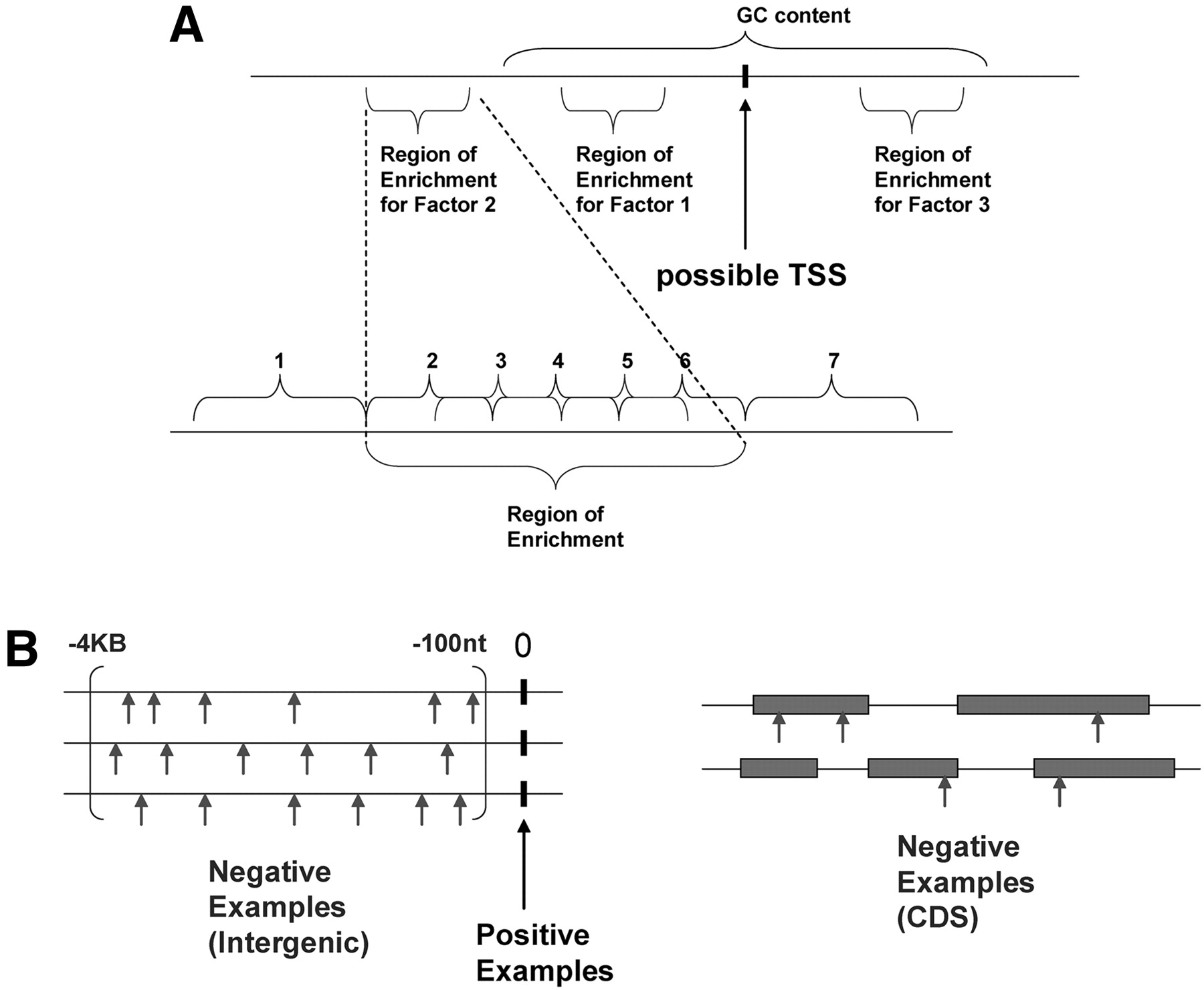
(A) For each example (location) considered, features are generated by adding up affinity scores for each TF within its region of enrichment. The lower portion of the diagram illustrates how this is done in detail: Each region is divided into five overlapping subwindows covering the region of enrichment, plus two flanking subwindows. Positive log-likelihood scores are summed over all positions in each subwindow, generating seven features for each TF. Additionally, GC content within a 100-nt region on either side of the location is also computed as a feature. The intuition behind this setup is to allow a trained model to select which elements and regions are most predictive of a TSS. (B) Training data sets are constructed from positive examples (the TSS locations themselves) and two types of negative examples: intergenic locations drawn at random from the immediate upstream regions of the TSS locations, and coding sequence examples drawn at random from annotated CDS regions on the mouse genome. Twenty intergenic locations are drawn from each immediate upstream region, and CDS locations are drawn in a 1:1 ratio with positive examples (to comprise ∼5% of the negative data set).