Abstract
Detailed modeling of a species’ history is of prime importance for understanding how natural selection operates over time. Most methods designed to detect positive selection along sequenced genomes, however, use simplified representations of past histories as null models of genetic drift. Here, we present the first method that can detect signatures of strong local adaptation across the genome using arbitrarily complex admixture graphs, which are typically used to describe the history of past divergence and admixture events among any number of populations. The method—called graph-aware retrieval of selective sweeps (GRoSS)—has good power to detect loci in the genome with strong evidence for past selective sweeps and can also identify which branch of the graph was most affected by the sweep. As evidence of its utility, we apply the method to bovine, codfish, and human population genomic data containing panels of multiple populations related in complex ways. We find new candidate genes for important adaptive functions, including immunity and metabolism in understudied human populations, as well as muscle mass, milk production, and tameness in specific bovine breeds. We are also able to pinpoint the emergence of large regions of differentiation owing to inversions in the history of Atlantic codfish.
One of the main goals of population genomics is to understand how adaptation affects patterns of variation across the genome and to find ways to analyze these patterns. To identify loci that have been affected by positive selection in the past, geneticists have developed methods that can scan a set of genomes for signals that are characteristic of this process. These signals may be based on patterns of haplotype homozygosity (Voight et al. 2006; Sabeti et al. 2007), the site frequency spectrum (Nielsen et al. 2005; Huber et al. 2016), or allelic differentiation between populations (Shriver et al. 2004; Yi et al. 2010).
Population differentiation–based methods have proven particularly successful in recent years, as they make few assumptions about the underlying demographic process that may have generated a selection signal, and are generally more robust and scalable to large population-wide data sets. The oldest of these are based on computing pairwise FST (Wright 1949; Weir and Cockerham 1984) or similar measures of population differentiation between two population panels across SNPs or windows of the genome (Lewontin and Krakauer 1973; Akey et al. 2002; Weir et al. 2005). More recent methods have allowed researchers to efficiently detect which populations are affected by a sweep, by computing branch-specific differentiation on three-population trees (Yi et al. 2010; Chen et al. 2010; Racimo 2016), four-population trees (Cheng et al. 2017), or arbitrarily large population trees (Bonhomme et al. 2010; Fariello et al. 2013; Librado and Orlando 2018) or by looking for strong locus-specific differentiation or environmental correlations, using the genome-wide population-covariance matrix as a null model of genetic drift (Coop et al. 2010; Günther and Coop 2013; Guillot et al. 2014; Gautier 2015; Villemereuil and Gaggiotti 2015).
Although some of these methods for detecting selection implicitly handle past episodes of admixture, none of them uses “admixture graphs” that explicitly model both divergence and admixture in an easily interpretable framework (Patterson et al. 2012; Pickrell and Pritchard 2012). This makes it difficult to understand the signatures of selection when working with sets of multiple populations that may be related to each other in complex ways. Here, we introduce a method to efficiently detect selective sweeps across the genome when analyzing many populations that are related via an arbitrarily complex history of population splits and mergers. We modified the QB statistic (Racimo et al. 2018), which was originally meant to detect polygenic adaptation using admixture graphs. Unlike QB, our new statistic—which we call SB—does not need gene-trait association data and works with allele frequency data alone. It can be used to both scan the genome for regions under strong single-locus positive selection and to pinpoint where in the population graph the selective event most likely took place. We show the usefulness of this statistic by performing selection scans on human, bovine, and codfish data, recovering existing and new candidate loci while obtaining a clear picture of which populations were most affected by positive selection in the past.
Results
Detecting selection on a graph
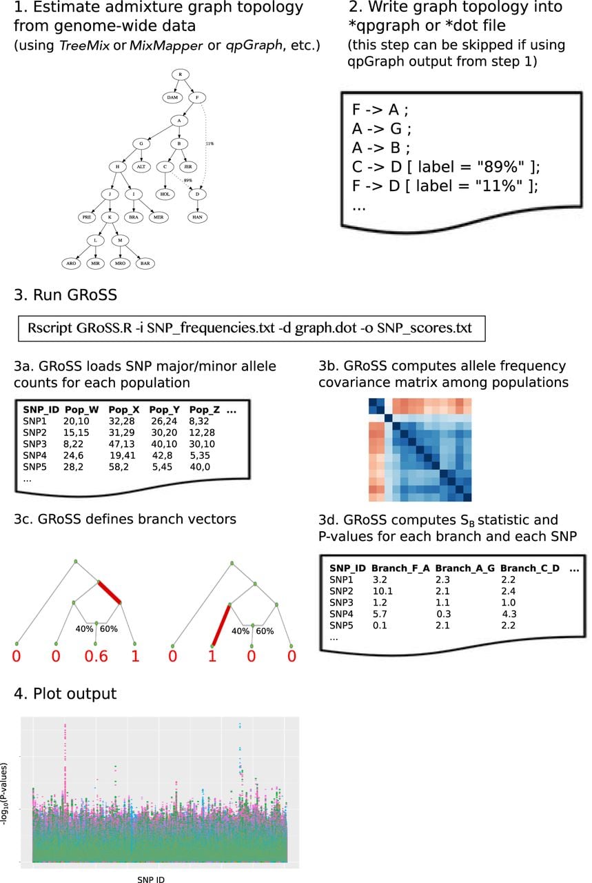
We modified the previously developed QB statistic (Racimo et al. 2018) to detect strong branch-specific deviations in single-locus allele frequencies but without having to use effect size estimates from an association study (see Methods section). We call our new statistic SB, and we implemented it in the program GRoSS, which stands for graph-aware retrieval of selective sweeps (Fig. 1). For each polymorphic site tested along the genome, the program outputs an approximately -distributed statistic and P-value for each branch of an admixture graph. The P-value is the probability that, when the neutral model is true for that branch, the statistic would be greater than or equal to the actual observed statistic. The statistic is based on the allele frequency pattern observed across different populations. Strong deviations from neutrality along a particular branch of the graph at a particular site will lead to high values of the corresponding branch-specific statistic at that site and to low P-values.
Simulations
We performed simulations on SLiM 2 (Haller and Messer 2017), and used ROC and precision-recall curves to evaluate the performance of our method under different demographic scenarios and to compare the behavior of our scores under selection and neutrality. We used neutral simulations (s = 0) as “negatives” and simulations under selection as “positives” and evaluated how different score cutoffs affected the precision, recall, true-positive rate, and false-positive rate. For each demographic scenario, we tested four selective sweep modes: using simulations under two different selection coefficients (s = 0.1 and s = 0.01) as cases and, for each of these, conditioning on establishment of the beneficial mutation at >5% frequency or at >1% frequency. Each branch of each graph had a diploid population size (Ne) of 10,000.
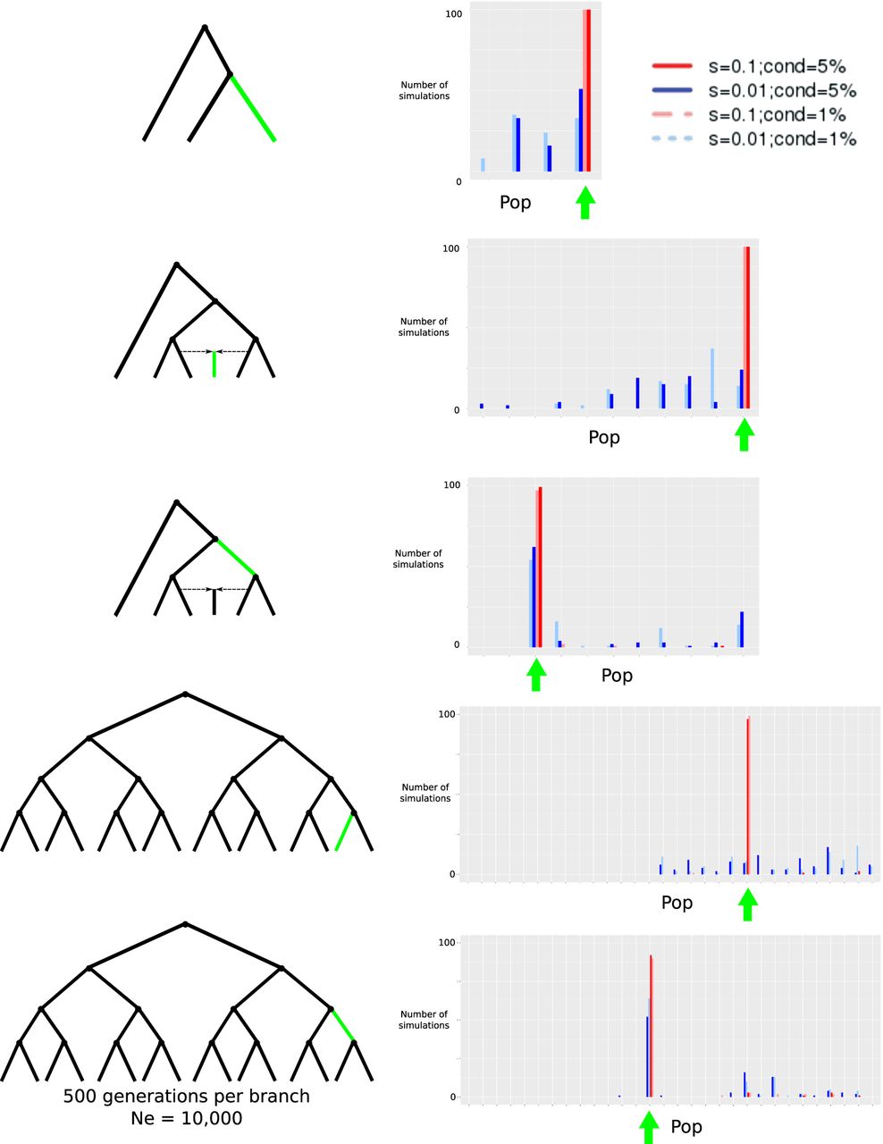
First, we simulated an episode of positive selection occurring on a branch of a three-population tree with no admixture. Each branch of the tree lasted for 500 generations. We sampled 100 individuals from each population. We applied our statistic in a region of 100 kb centered on the beneficial mutation, and kept track of which branch in each simulation had the highest score. As shown in Figure 2, the highest values typically correspond to the population in which the selected mutation was introduced. The performance of the method under both selection coefficients is better when we condition on a higher frequency of establishment of the beneficial allele, and is also better under strong selection (Fig. 3).
Evaluation of GRoSS performance using simulations in SLiM 2, with 100 diploid individuals per population panel. We simulated different selective sweeps under strong (s = 0.1) and intermediate (s = 0.01) selection coefficients for a three-population tree, a six-population graph with a 50%/50% admixture event, and a 16-population tree. We obtained the maximum branch score within 100 kb of the selected site and computed the number of simulations (out of 100) in which the branch of this score corresponded to the true branch in which the selected mutation arose (highlighted in green). (cond = 5%) Simulations conditional on the beneficial mutation reaching 5% frequency or more; (cond = 1%) simulations conditional on the beneficial mutation reaching 1% frequency or more; (Pop) population branch. The green arrow denotes the values of the statistic corresponding to the branch in which the selected mutation arose.
Evaluation of GRoSS performance using simulations in SLiM 2, with 100 diploid individuals per population panel. We produced precision-recall (left) and ROC (center and right) curves comparing simulations under selection to simulations under neutrality for a three-population tree, a six-population graph with a 50%/50% admixture event, and a 16-population tree. The right-most ROC curves are a zoomed-in version of the center ROC curves, in which the false-positive rate is limited to be equal to or less than 0.1.
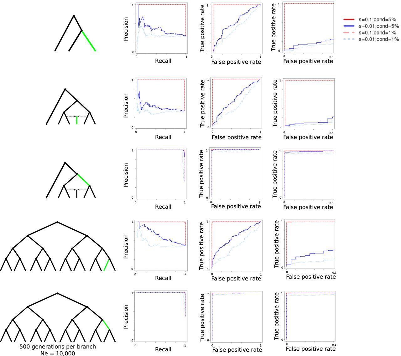
We also simulated more complex demographic histories, including a six-population graph with admixture. Each branch of the graph lasted for 500 generations. We explored two different selection scenarios. In one scenario, the selective sweep was introduced in one of the internal branches, whereas in another scenario, it was introduced in one of the external branches. The performance under this graph appears to improve relative to the three-population scenario (Fig. 3). The reason is that the SB statistic depends on having an accurate estimate of the ancestral allele frequency (e). This estimate is calculated by taking the average of all allele frequencies in the leaf populations; so the more leaf populations in a well-balanced graph we have, the more accurate this estimate will be. We also explored a larger population tree with 16 leaf populations. ROC and precision-recall curves show a similar performance to the ones from the six-population admixture graph (Fig. 3). The method performs slightly worse if the selected mutation is introduced in a terminal branch than in an upper branch of the graph, because the selected mutation has more time to keep rising in frequency in daughter populations, if it is simulated earlier in the process.
In addition, we explored the performance of the method when the number of diploid individuals per population was smaller than 100. Supplemental Figures S1 and S2 show the performance of the method with 50 diploid individuals per population, Supplemental Figures S3 and S4 show the performance with 20 individuals, and Supplemental Figures S5 and S6 show the performance with four individuals. Even when the number of individuals is this small, we can still recover most of the simulated sweeps, especially when selection is strong. The performance of the method also remains robust if the different population panels have highly different sample sizes (Supplemental Figs. S7, S8).
The assumption of constant population size might not be realistic for most real-world applications. For this reason, we simulated a 5× bottleneck lasting 10 generations in two different parts of the six-population graph. In this situation, GRoSS is still able to identify the true branch in which the selected mutation arose (Supplemental Fig. S9). Under a range of sample sizes, the method performs similarly to the case without a bottleneck (Supplemental Figs. S10–S13).
Finally, we tested the effects of graph misspecification by simulating selection under a six-population graph with one admixture event but then feeding GRoSS two different topologies that were different from the simulated topology. A direct comparison of performance to the true topology case is impossible given that there is not a one-to-one correspondence between the branches of the correct graph and the wrong graphs. However, we generally find that the branch in the wrong graphs that completely subtends the populations that are also subtended by the selected branch in the correct graph is the one in which selection is inferred to have occurred most of the time (Supplemental Fig. S14). This occurs for all sample size scenarios with the exception of the case in which sample sizes are very low across the graph (n = 4 in all terminal leaves).
Positive selection in human populations across the world
We applied our method to a whole-genome data set (The 1000 Genomes Project Consortium 2015) and a SNP capture data set (Human Origins) (Patterson et al. 2012) from different populations sampled around the world (Fig. 4) and obtained the top candidate regions from the scan (P-value < 10−7). Many of these have been identified in previous world-wide positive selection scans, and some have evidence for archaic adaptive introgression. Previously reported selection candidates that are among the top regions include LCT/MCM6, BNC2, OCA2/HERC2, TLR, and SLC24A5 regions in northern Europeans; the CHMP1A/ZNF276/FANCA, ABCC11, and POU2F3 regions in East Asians; and the SLC45A2 and SLC12A1 genes in an ancestral European population (Supplemental Tables S2, S3; Bersaglieri et al. 2004; Voight et al. 2006; Chen et al. 2010; Ohashi et al. 2011; Grossman et al. 2013; Vernot and Akey 2014; Mathieson et al. 2015; Racimo 2016; Racimo et al. 2016).
We ran GRoSS on human genomic data. (A) Population tree including panels from phase 3 of the 1000 Genomes Project. (B) Population graph including imputed panels from the Human Origins SNP capture data from Lazaridis et al. (2014).
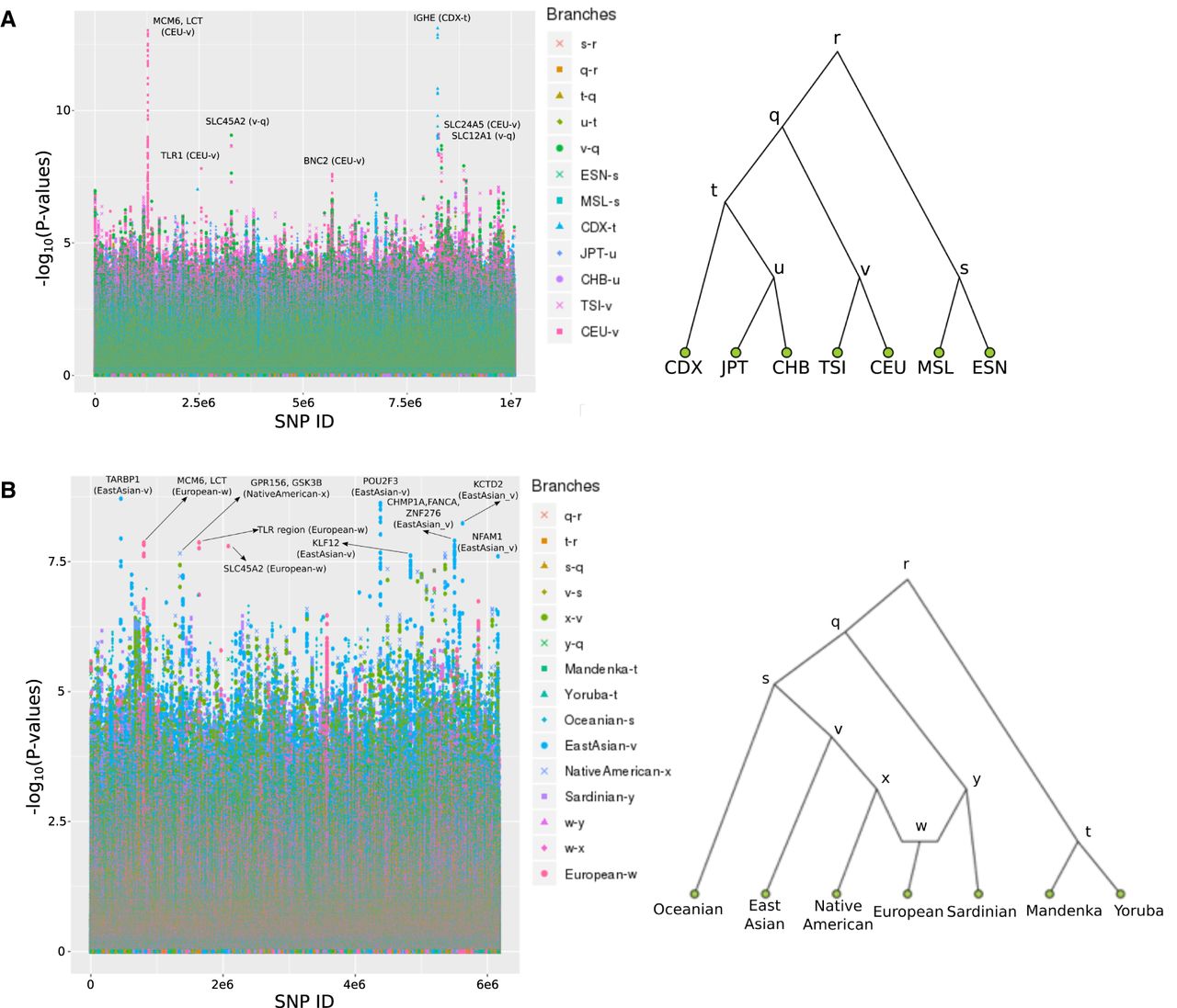
We find that the IGH immune gene cluster (also containing gene FAM30A) is the strongest candidate for selection in the 1000 Genomes scan, and the signal is concentrated on the Chinese Dai branch. This cluster has been recently reported as being under selection in a large Chinese cohort of more than 140,000 genomes (Liu et al. 2018). Our results suggest that the selective pressures may have existed somewhere in southern China, as we do not see such a strong signal in other parts of the East Asian portion of the graph.
A region containing TARBP1 is the strongest candidate for selection in the Human Origins scan (East Asian terminal branch). The gene codes for an HIV-binding protein and has been previously reported to be under balancing selection (Andrés et al. 2009). The top SNP (rs2175591) lies in an H3K27ac regulatory mark upstream of the gene. The derived allele at this SNP is at >50% frequency in all 1000 Genomes East Asian panels but is at <2% frequency in all the other worldwide panels, except for South Asians, where it reaches frequencies of ∼10%. The TARBP1 gene has been identified as a target for positive selection in milk-producing cattle (Stella et al. 2010) and in sheep breeds (de Simoni Gouveia et al. 2017; Mastrangelo et al. 2018). It has also been associated with resistance to gastrointestinal nematodes in sheep (Keane et al. 2006). Our results suggest it may have also played an important role during human evolution in eastern Eurasia, possibly as a response to local pathogens.
Another candidate for selection is the NFAM1 gene in East Asians, which codes for a membrane receptor that is involved in development and signaling of B cells (Ohtsuka et al. 2004). This gene was also found to be under positive selection in the Sheko cattle of Ethiopia, along with other genes related to immunity (Bahbahani et al. 2018).
In the Native American terminal branch of the Human Origins scan, we find a candidate region containing two genes: GPR156 and GSK3B. GPR156 codes for a G protein–coupled receptor, whereas GSK3B codes for a kinase that plays important roles in neuronal development, energy metabolism, and body pattern formation (Plyte et al. 1992). We also find a candidate region in the same branch in the protamine gene cluster (PRM1, PRM2, PRM3, TNP2), which is involved in spermatogenesis (Schlüter et al. 1992; Engel et al. 1992), and another region overlapping MDGA2, which is specifically expressed in the nervous system (Litwack et al. 2004).
Cattle breeding: morphology, tameness, and milk yield
We also applied GRoSS to a data set containing various cattle populations from around the world (Supplemental Table S4; Kim et al. 2017; Upadhyay et al. 2017; da Fonseca et al. 2019). We performed two scans, one in which we computed the SB statistic per SNP (Supplemental Table S5; Fig. 5) and one in which we computed it in 10-SNP windows (Supplemental Table S6; Fig. 5). Out of the 12 top candidate regions, 10 overlapped with regions previously detected to be under selection in cattle (for review, see Randhawa et al. 2016). Additionally, 28 of the 43 top candidate SNPs from the single-SNP scan are also in regions that have been previously reported as selection candidates.
We ran GRoSS on a population graph of bovine breeds. P-values were obtained either (1) by computing chi-squared statistics per SNP, or (2) after averaging the per-SNP statistics in 10-SNP windows with a 1-SNP step size, obtaining a P-value from the averaged statistic. Holstein and Maremmana cattle photos obtained from Wikimedia Commons (authors: Verum; Giovanni Bidi). Romanian Grey cattle screen-shot obtained from a CC-BY YouTube video (author: Paolo Caddeo).
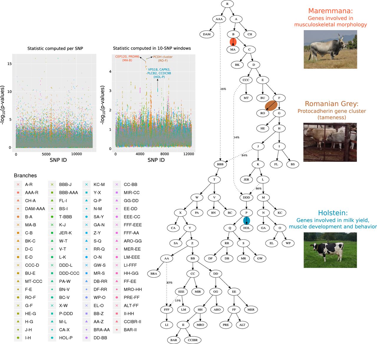
The region located between 50 and 55 Mb contains three members of the protocadherin gene cluster (Pcdha, Pcdhb, and Pcdhg) (Fig. 6). The SB statistic is highest in Romanian Grey (RO) cattle, which are well-known for their docile disposition. Protocadherins are cell-adhesion molecules that are differentially expressed in individual neurons (Chen and Maniatis 2013). They have been implicated in mental retardation and epilepsy in humans (Hayashi and Takeichi 2015) and in fear-conditioning and memory in mice (Fukuda et al. 2008) and have also been shown to be under selection in cats (Montague et al. 2014). Genes of the protocadherin family have also been detected to have expression and allele frequency differences consistent with adaptation in an analysis of tame and aggressive foxes (Wang et al. 2018).
Zoomed-in plots of GRoSS output for three regions found to have strong evidence for positive selection in the 10-SNP bovine scan. Genes were retrieved using Ensembl via the Gviz R Bioconductor library (Hahne and Ivanek 2016).
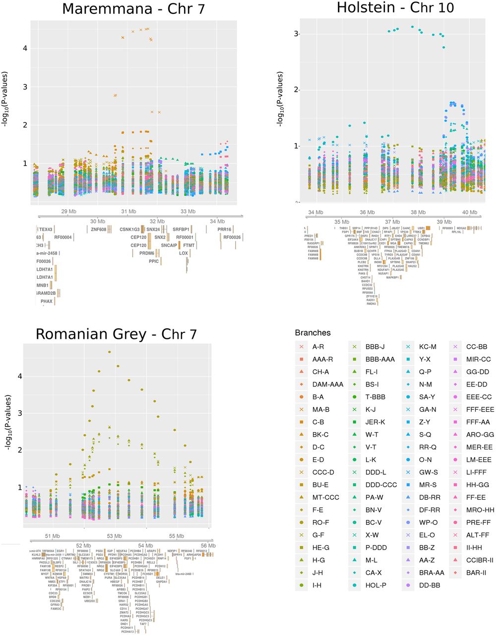
The largest window (4.4 Mb) detected by GRoSS corresponds to the branch leading to the Holstein (HOL) breed (Fig. 6). This window overlaps regions found to be under selection in HOL using various tests (for review, see Randhawa et al. 2016). Some of the outlier genes that were also identified in an earlier XP-EHH scan (Lee et al. 2014) include VPS18, implicated in neurodegeneration (Peng et al. 2012), and CAPN3, associated with muscle dystrophy. The window also contains genes that are differentially expressed between high and low milk yield cows (PLCB2 and CCDC9B) (Yang et al. 2016).
Large regions of extreme differentiation in Atlantic codfish
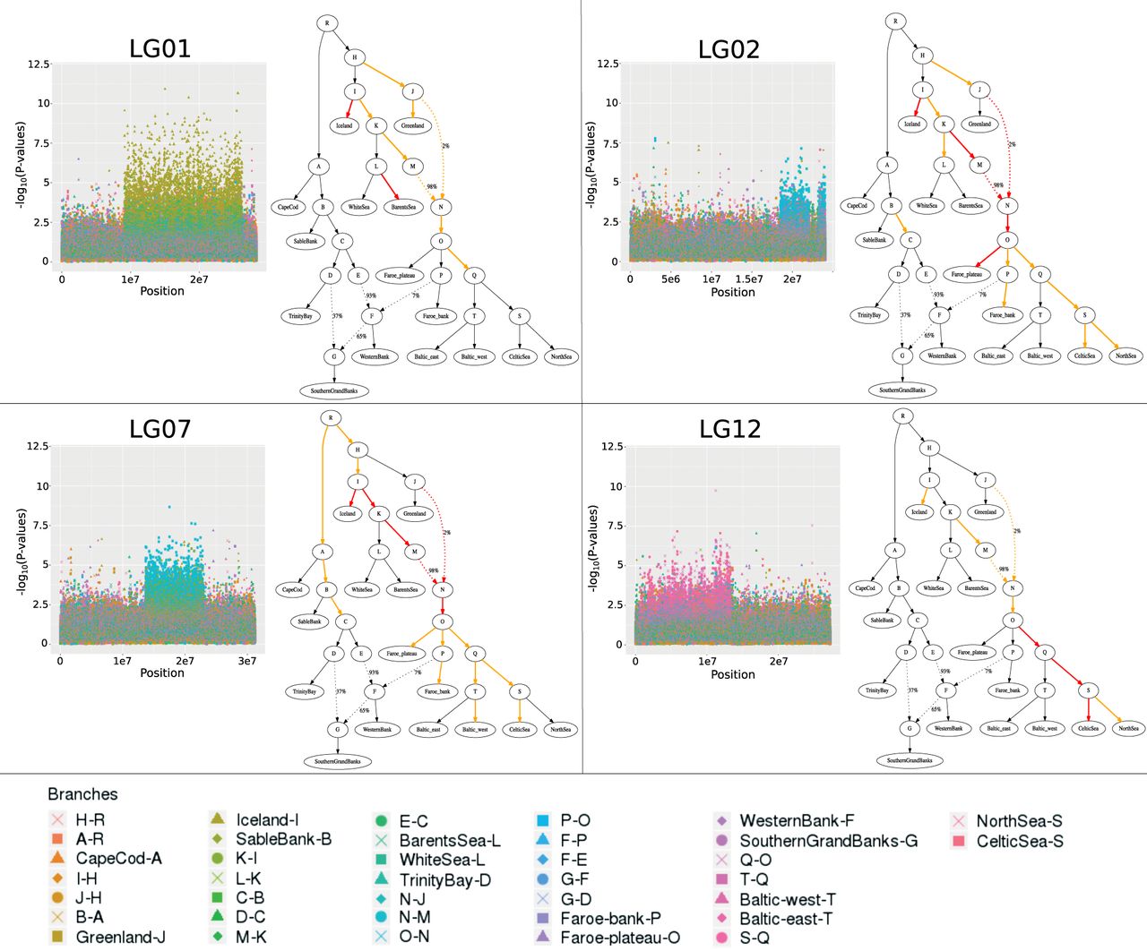
Finally, we applied GRoSS to a data set of Atlantic codfish genomes (Supplemental Table S7; Árnason and Halldórsdóttir 2019). We find four large genomic regions of high differentiation spanning several megabases, on four different linkage groups: LG01, LG02, LG07, and LG12 (Fig. 7; Supplemental Table S8). These regions were previously detected by pairwise FST analyses (Bradbury et al. 2013; Hemmer-Hansen et al. 2013; Halldórsdóttir and Árnason 2015). They are associated with inversions that suppress recombination in heterozygous individuals and have thereby favored large increases in differentiation between haplotypes. The signals in the LG01, LG02, and LG07 regions are strongest among north Atlantic populations. The LG01 signal is particularly concentrated in the terminal branches leading to the Icelandic and Barents Sea populations. The LG02 signal is concentrated in the Icelandic terminal branch and the parent branches of the east Atlantic/north European populations. This region also contains a low-differentiation region inside it, suggesting it may be composed of two contiguous structural variants, as the LG01 region is known to be (Kirubakaran et al. 2016). The LG07 signal is concentrated in nearly the same branches as the LG02 signal and also in the Faroe plateau terminal branch. In contrast, the highly differentiated region in LG12 is concentrated among other branches of the east Atlantic/north European part of the graph, including the Celtic Sea terminal branch (Fig. 7). None of the highly differentiated regions appears to show strong signs of high differentiation in the west Atlantic/North American populations.
Large regions of high differentiation in the codfish data. Branches colored in orange are branches whose corresponding SB scores evince the high-differentiation region. Branches colored in red are branches whose corresponding SB scores evince the high-differentiation region and have at least one SNP with −log10 (P) > 5 inside the region.
Discussion
We have developed a method for detecting positive selection when working with species with complex histories. The method is fast: It only took 486 sec to run the bovine scan (including 512,358 SNPs and 36 populations) on a MacBook Air with a 1.8-GHz Intel Core i5 processor and 8 GB of memory. Assuming a null model of genetic drift based on a multivariate normal distribution, the SB statistic is chi-squared distributed with one degree of freedom. This is accurate as long as the graph topology is accurate and the branches in the graph do not contain high amounts of drift. When working with populations that diverged from each other a long time ago, the chi-squared distributional assumption will not hold, and in those cases, it may be useful to standardize the scores using the mean and variance of the empirical genome-wide distribution.
In an admixture graph with K branches, there are K possible versions of the SB statistic. If the differences in allele frequencies at a SNP can be explained by an allele frequency shift that occurred along branch k, then SB (k) will be large, and a P-value based on the null drift model can be calculated from it. By design, branches whose parent are the root node and branches that have the same descendant nodes have the same SB scores, so selective events on these branches are not distinguishable from each other under this scheme.
It is important to emphasize that GRoSS works on the assumption that the graph is a good descriptor of the ancestry relationships among populations, which are coded in the genome-wide covariance matrix . We expect a reduction in power relative to methods that directly use the raw covariance matrix to assess the evidence for positive selection (Coop et al. 2010; Günther and Coop 2013; Guillot et al. 2014; Gautier 2015; Villemereuil and Gaggiotti 2015) if the population history does not follow a graph-like pattern. This is the cost of the higher interpretability of GRoSS. The former methods can only serve to determine whether the population allele frequencies at a site are poorly modeled by or whether they are better explained by environmental covariates, whereas GRoSS can provide a historical interpretation of positive selection in terms of allele frequency shifts at particular branches of the population history.
We compare GRoSS against one of the most powerful members of this family of covariance matrix-based programs, BayPass, in Supplemental Figure S15 (lower panel). Here, we plot a scan of a selective sweep using the XtX statistic from BayPass (based on the Bayenv model [Coop et al. 2010]) (Gautier 2015), which works similarly to GRoSS but without a graph model. We observe that BayPass has good power to detect the sweep but provides a single score and therefore cannot be used by the user to localize when in the population history the sweep took place. Furthermore, if one compares the XtX statistic under selection and neutrality (Supplemental Fig. S16) with the SB statistic under selection (in the true selected branch) and neutrality (Fig. 3), one can see that GRoSS actually outperforms BayPass at detecting selection. In summary, assuming that a graph is a good descriptor of the population history and that GRoSS has correctly identified the true branch under selection, then the GRoSS branch-specific score performs better than the XtX score, which cannot indicate which part of the history was under selection.
The SB statistic is most accurate when a large number of individuals have been sampled from each population. If this is not the case, then one can merge sister populations into larger populations, so as to increase the per-population sample size. Another option is to average the scores over windows of SNPs to obtain power from correlated allele frequency shifts in a region (e.g., see Akey et al. 2002; Skoglund et al. 2017) at the expense of losing spatial resolution across the genome owing to larger test regions, as we did here in the bovine data set example. The statistic, however, does not account for the structure of linkage disequilibrium within or between windows.
We have found the method performs best when there are many leaves in a graph because it uses a population-averaged allele frequency to estimate the ancestral allele frequency in the graph. We therefore recommend using this method when working with more than a few populations at a time to make this estimate as accurate as possible. A possible future improvement of the method could be the incorporation of a model-based ancestral allele frequency estimation scheme to address this issue. For example, to more appropriately account for the population covariance structure, we could use the unbiased linear estimate of e with minimum variance, (Bonhomme et al. 2010). However, we found this estimate generates an excess of significant P-values when working with allele frequencies at the boundaries of fixation and extinction or when there are several populations in which the SNP is not segregating, owing to poor modeling of frequency dynamics by the multivariate normal distribution. Previous applications of these types of methods have also replaced the ancestral allele frequency by the mean population frequency (Berg and Coop 2014; Berg et al. 2017a), as we did, or simply use models without a root (Yi et al. 2010).
Another critical issue is that the more branches one tests, the more of a multiple-testing burden there will be when defining significance cutoffs. In a way, our method improves on previous approaches to this problem because, given an inferred admixture graph, one does not need to perform a test for all possible triplets or pairs of populations, as one would need to do when applying the PBS statistic (Yi et al. 2010) or pairwise FST methods (Wright 1949; Weir and Cockerham 1984), respectively. Instead, our method performs one test per branch. For example, if the graph is a rooted tree with m leaves and no admixture, the number of branches will be equal to 2m − 2, whereas the number of possible PBS tests will be equal to , and the number of possible pairwise FST tests will be equal to , both of which grow much faster with larger m than does 2m − 2. When working with a multipopulation graph, this leaves the potential user with the only option of calculating a battery of tests, some of which detect the sweep and some of which do not.
To further illustrate this point, in Supplemental Figure S15 we show how pairwise FST, PBS, and GRoSS can be used to detect a single selective sweep (s = 0.1) in two different branches of a six-population graph. Neither FST nor PBS uses an admixture graph model. Pairwise FST works by simply calculating the FST statistic between two populations but cannot distinguish which was the population that underwent a sweep. PBS is a linear combination of log-transformed FST values that allows one to localize the sweep to one of the branches of a three-branch unrooted tree. However, as stated before, the number of possible PBS tests grows very fast with the number of populations, indeed faster than the number of FST tests. In Supplemental Figure S15, we only plot the 15 possible FST tests that could be run on the depicted graph. There are 60 possible PBS tests that we could have run on this same graph, but we only show three of these, configured in a way that we knew a priori that only one test would contain the selected branch. Although it is clear that both PBS and FST have good power to detect the sweep, it is also clear that it would be a herculean task to visually infer the true branch in which the selected mutation arose from all of the possible PBS or FST tests one could run in a graph.
Although the SB statistic is fast and easy to compute, it is not as principled as other approaches for multipopulation selection that rely on explicit models of positive selection (e.g., Lee and Coop 2017). This means that it only detects significant deviations from a neutral null model and does not provide likelihoods or posterior probabilities supporting specific selection models. We recommend that, once a locus with high SB has been detected in a particular branch of a graph, biologists should perform further work to disentangle exactly what type of phenomenon would cause this value to be so high and to test among competing selection hypotheses.
Among the genes that emerge when applying our method to human data, we found several known candidates, like LCT/MCM6, SLC45A2, SLC24A5, POU2F3, OCA2/HERC2, and BNC2. We also found several new candidate regions, containing genes involved in the immune response, like the TARBP1 and NFAM1 genes in East Asians. Additionally, we found new candidate regions in Native Americans, like GSK3B and the protamine gene cluster.
Analysis of the bovine data set yielded numerous regions that may be implicated in the breeding process. One of the strongest candidate regions contains genes involved in musculoskeletal morphology, including CEP120 and PRDM6, and GRoSS narrows this signal down to the branch leading to the Maremmana breed. This is an Italian beef cattle breed that inhabits the Maremma region in Central Italy and has evolved a massive body structure well adapted to draft use in the marshy land that characterizes the region (Bongiorni et al. 2016). When comparing muscle samples between Maremmana and the closely related Chianina (CH) breed, Gene Ontology categories related to muscle structural proteins and regulation of muscle contraction have been reported to be enriched for differentially expressed genes. Additionally, the Maremmana is enriched for overexpressed genes related to hypertrophic cardiomyopathy pathways (Bongiorni et al. 2016).
Another strong candidate region is the protocadherin gene cluster, associated with neuronal functions in humans and mice (Fukuda et al. 2008; Chen and Maniatis 2013; Hayashi and Takeichi 2015) and shown to be under positive selection in domesticated cats and foxes (Montague et al. 2014; Wang et al. 2018). GRoSS identifies this region as under selection in the RO breed terminal branch. Given that this breed is popularly known to be very docile, it is plausible that this gene cluster might have been a target for selection on behavior during the recent breeding process.
Additionally, GRoSS detects a very large 4.4-Mb region as a selection candidate in the HOL breed, currently the world's highest-production dairy animal. This region overlaps several candidate genes earlier identified to be under selection in HOL using other methods (for an extensive review, see Randhawa et al. 2016). These genes are related to several traits usually targeted by breeding practices, such as behavior, muscle development, and milk yield.
Our method also recovered previously reported regions of high differentiation among Atlantic codfish populations and served to pinpoint where in the history of this species the inversions may have arisen or, at least, where they have most strongly undergone the process of differentiation between haplotypes. The largest of these regions is in LG01 and is composed of two adjacent inversions covering 17.4 Mb (Kirubakaran et al. 2016), which suppress recombination in heterozygous individuals and promote differentiation between haplotypes. The inversions effectively lock together a supergene of alleles at multiple loci (Kirubakaran et al. 2016). Two behavioral ecotypes—a deep-sea frontal (migratory) ecotype and a shallow-water coastal (stationary) ecotype—have been associated with inversion alleles in the region (Pálsson and Thorsteinsson 2003; Pampoulie et al. 2008; Thorsteinsson et al. 2012). Several putative candidate selected genes are located within the LG01 inversions (Pogson 2001; Pampoulie et al. 2015; Kirubakaran et al. 2016) that may be of adaptive value for deep sea as well as long-distance migration.
Similarly, the other large inversions observed in linkage groups LG02, LG07, and LG12 (5, 9.5, and 13 Mb, respectively) also suppress recombination (Sodeland et al. 2016; Berg et al. 2017b). Allele frequency differences observed between individuals living offshore and inshore environments are suggestive of ecological adaptation driving differentiation in these regions (Sodeland et al. 2016; Berg et al. 2017b; Barth et al. 2017). Previously, a pairwise FST outlier analysis of populations in the north (Greenland, Iceland, and Barents Sea localities combined) versus populations in the south (Faroe Islands, North Sea, and Celtic Sea combined) showed clear evidence of selection in these regions (Halldórsdóttir and Árnason 2015). However, in comparisons of west (Sable Bank, Western Bank, Trinity Bay, and Southern Grand Banks combined) with either north or south localities, only some of these regions displayed signatures of high differentiation (Halldórsdóttir and Árnason 2015), indicating these inversions had different spatiotemporal origins. By modeling all these populations together in a single framework, our method provides a way to more rigorously determine in which parts of the graph these inversions may have originated (Fig. 7) and suggests they were largely restricted to East Atlantic populations.
In conclusion, GRoSS is a freely available, fast, and intuitive approach to testing for positive selection when the populations under study are related via a history of multiple population splits and admixture events. It can identify signals of adaptation in a species by accounting for the complexity of this history while also providing a readily interpretable score. This method will help evolutionary biologists and ecologists pinpoint when and where adaptive events occurred in the past, facilitating the study of natural selection and its biological consequences.
Methods
Theory
We assume that the topology of the admixture graph relating a set of populations is known and that we have allele frequency data for all the populations we are studying. For a single SNP, let p be the vector of allele frequencies across populations. We then make a multivariate normal approximation to obtain a distribution with which we can model these frequencies under neutrality (Nicholson et al. 2002; Bonhomme et al. 2010; Coop et al. 2010; Günther and Coop 2013):
We then obtain a mean-centered version of the vector p, which we call y:
Then, standardizing the square of yTb yields a chi-squared-distributed statistic:
Our test statistic—which we call SB—is therefore defined as
If we only have a few genomes per population, the true population allele frequencies will be poorly estimated by our sample allele frequencies, potentially decreasing power. However, we can increase power at the cost of spatial genomic resolution and rigorous statistical interpretation by combining information from several SNPs into windows (Akey et al. 2002; Skoglund et al. 2017). We can compute the average χ2 statistic over all SNPs in each window and provide a new P-value for that averaged statistic.
Implementation
We implemented the SB statistic in a program called graph-aware retrieval of selective sweeps (GRoSS) that uses the R statistical language (R Core Team 2019). The program makes use of the admixturegraph library (Leppälä et al. 2017). We also wrote a module that allows one to input a file specifying the admixture graph topology directly.
Figure 1 shows a schematic workflow for GRoSS. The user begins by estimating an admixture graph using genome-wide data, via a program like TreeMix (Pickrell and Pritchard 2012), MixMapper (Lipson et al. 2013), or qpGraph (Patterson et al. 2012). Then the user writes the topology of the graph to a text file. The format of this file can be either the dot-format or the input file format for qpGraph, so it can be skipped if the initial step was run using qpGraph. Then, the user inputs the graph topology and a file with major/minor allele counts for each SNP into GRoSS. The allele counts can also be polarized as ancestral/derived or reference/alternative. GRoSS will compute the genome-wide covariance matrix and the b vectors for each branch and then will calculate the SB scores and corresponding P-values, which can then be plotted.
Simulations
We used SLiM 2 (Haller and Messer 2017) to simulate genomic data and test how our method performs at detecting positive selection, with sample sizes of 100, 50, 25, and four diploid genomes per population (Figs. 2, 3; Supplemental Figs. S1–S6). Unless otherwise stated, we simulated a genomic region of length 10 Mb, a constant effective population size (Ne) of 10,000, a mutation rate of 10−8 per base-pair per generation, and a uniform recombination rate of 10−8 per base-pair per generation. We placed the beneficial mutation in the middle of the region, at position 5 Mb. We used a burn-in period of 100,000 generations to generate steady-state neutral variation. For each demographic scenario that we tested, we simulated under neutrality and two selective regimes, with selection coefficients (s) of 0.1 and 0.01. We considered two types of selection scenarios for each demographic scenario: one in which we condition on the beneficial mutation reaching >1% frequency at the final generation of the branch in which we simulated the beneficial mutation and one in which we condition the mutation reaching >5% frequency. We discarded simulations that did not fulfill these conditions. We set the time intervals between population splits at 500 generations for all branches of the population graph in the three-population, six-population, and 16-population graphs. To speed up the simulations, we scaled the values of the population size and of time by a factor of 1/10 and, consequently, the mutation rate, recombination rate, and selection coefficients by a factor of 10 (Haller and Messer 2017).
Selection of candidate regions
Given the myriad of plausible violations of our null multivariate-normal model (see Discussion), we do not expect the P-values of the SB statistic to truly reflect the probability one has of rejecting a neutral model of evolution. To show this, we assessed the fit of our SB statistic under neutrality to the expected chi-squared distribution, using density plots and qq-plots. We simulated a six-population graph with one admixture event and sampled 100, 50, 25, or four genomes from each population (Supplemental Figs. S17–S20, respectively). Although the score and chi-squared distributions are quite close to each other for almost all branches, they are not a perfect fit. Thus, users should be careful about using these P-values at face value. In Supplemental Table S1, we show the proportion of observations that are larger than the chi-squared statistic that would correspond to a particular P-value cutoff for different choices of cutoffs.
We therefore see these P-values as a guideline for selecting regions as candidates for positive selection rather than a way for rigorously determining the probability that a region has been evolving neutrally. In all applications below, we used arbitrary P-value cutoffs to select the top candidate regions. These empirical cutoffs vary across study species and also depend on the specific scheme we use to calculate the SB statistic (per-SNP or averaged over a window), and we do not claim these cutoffs to have any statistical motivation beyond being convenient ways to separate regions that lie at the tails of our empirical distribution.
Alternative approaches could involve using a randomization scheme or generating simulations based on a fitted demographic model to obtain a neutral distribution of loci and derive a P-value from that. Although any of those approaches could be pursued with the SB framework, we do not pursue any of those approaches in this paper. We think that the chosen mode of randomization or the fitted demographic parameters will also necessarily rely on assumptions about unknown or unmodeled parameters and may provide unmerited confidence to the cutoff that we could end up choosing. Instead, we recommend that our chi-squared-distributed P-values are utilized as a way to prioritize regions for more extensive downstream modeling and validation (e.g., using methods like those described by Akbari et al. 2018; Kern and Schrider 2018; Sugden et al. 2018).
GRoSS users should also be mindful of multiple testing and use statistical corrections that account for the fact that a selection scan involves testing multiple sites across the genomes, which may not be independent owing to linkage. In the particular case of GRoSS, if one is testing for selection across multiple branches of a complex graph, one should also aim to correct for multiple testing across branches.
Human data
We used data from Phase 3 of the 1000 Genomes Project (The 1000 Genomes Project Consortium 2015) and a SNP capture data set of present-day humans from 203 populations genotyped with the Human Origins array (Patterson et al. 2012; Lazaridis et al. 2014). The SNP capture data set was imputed using SHAPEIT2 (Delaneau et al. 2013) on the Michigan Imputation Server (Das et al. 2016) with the 1000 Genomes data as the reference panel (Racimo et al. 2018). We used inferred admixture graphs that were fitted to this panel using MixMapper (v1.02) (Lipson et al. 2013) in a previous publication (Racimo et al. 2018). For the 1000 Genomes data set, the inferred graph was a tree in which the leaves are composed of panels from seven populations: Southern Han (CDX), Han Chinese from Beijing (CHB), Japanese from Tuscany (JPT), Toscani (TSI), Utah Residents (CEPH) with Northern and Western European Ancestry (CEU), Mende from Sierra Leone (MSL), and Esan from Nigeria (ESN) (Fig. 4). For the Human Origins data set, the inferred graph was a seven-leaf admixture graph that includes Native Americans, East Asians, Oceanians, Mandenka, Yoruba, Sardinians, and Europeans with high ancient-steppe (Yamnaya) ancestry (Fig. 4). This graph contains an admixture event from a sister branch to Sardinians and a sister branch to Native Americans into Europeans; the latter represents the ancient steppe ancestry known to be present in almost all present-day Europeans (but largely absent in present-day Sardinians).
We removed sites with <1% minor allele frequency or where at least one population had no coverage. We then ran GRoSS on the resulting SNPs in each of the two data sets (Supplemental Tables S2, S3). We selected SNPs with −log10 (P) larger than seven and merged SNPs into regions if they were within 100 kb of each other. Finally, we retrieved all HGNC protein-coding genes that overlap each region, using biomaRt (Durinck et al. 2009).
Bovine data
We assembled a population genomic data set (Supplemental Table S4) containing different breeds of Bos taurus using (1) SNP array data from Upadhyay et al. (2017), corresponding to the Illumina BovineHD Genotyping BeadChip (http://dx.doi.org/10.5061/dryad.f2d1q); (2) whole-genome shotgun data from 10 individuals from the indigenous African breed NĎama (BioProject ID: PRJNA312138) (Kim et al. 2017); (3) shotgun data from two commercial cattle breeds (HOL and Jersey; BioProject IDs: PRJNA210521 and PRJNA318089, respectively); and (4) shotgun data for eight Iberian cattle breeds (da Fonseca et al. 2019).
We used TreeMix (Pickrell and Pritchard 2012) to infer an admixture graph (Supplemental Fig. S21) using allele counts for 512,358 SNPs in positions that were unambiguously assigned to the autosomes in the cattle reference genome version UMD3.1.1 (The Bovine Genome Sequencing and Analysis Consortium et al. 2009) using SNPchiMp (Nicolazzi et al. 2015). For shotgun data, allele counts were obtained from allele frequencies calculated in ANGSD (Korneliussen et al. 2014) for positions covered in at least three individuals. We removed SNPs for which at least one panel had no coverage or in which the minor allele frequency was <1%.
We ruled out the possibility that the intersection of shotgun and SNP capture data could be problematic by fitting a TreeMix tree using data from both approaches for the same breeds where available. No batch effects were observed (Supplemental Fig. S22), and in the end, we chose the type of data for which there were more individuals sequenced for each breed.
We applied the statistic to the TreeMix-fitted graph model in Figure 5. We performed the scan in two ways: In one, we computed a per-SNP chi-squared statistic, from which we obtained a P-value (Supplemental Table S5), and in the other, we combined the chi-squared statistics in windows of 10 SNPs (Supplemental Table S6), with a step size of one SNP, obtaining a P-value for a particular window using its average SB score (Fig. 5). We used this windowing scheme because of concerns about small sample sizes in some of the populations and because we aimed to pool information across SNPs within a region. After both scans, we combined windows that were within 100 kb of each other into larger regions and retrieved HGNC and VGNC genes within a ±100-kb window around the boundaries of each region using biomaRt (Durinck et al. 2009) with the April 2018 version of Ensembl.
Codfish data
Codfish genomes were obtained from Halldórsdóttir and Árnason (2015) and Árnason and Halldórsdóttir (2019). These were randomly sampled from a large tissue sample database (Árnason and Halldórsdóttir 2015) and the J. Mork collections from populations covering a wide distribution from the western Atlantic to the northern and eastern Atlantic (Supplemental Fig. S23; Supplemental Table S7). The populations differ in various life-history and other biological traits (Jakobsson et al. 1994; ICES 2005), and their local environment ranges from shallow coastal water (e.g., western Atlantic and North Sea) to waters of great depth (e.g., parts of Iceland and Barents Sea). They also differ in temperature and salinity (e.g., brackish water in the Baltic). Details of the molecular and bioinformatic methods used to obtain these genomes are given by Halldórsdóttir and Árnason (2015) and Árnason and Halldórsdóttir (2019).
We ran ANGSD (Korneliussen et al. 2014) on the genome sequences from all populations, computed base-alignment quality (Li 2011), adjusted mapping quality for excessive mismatches, and filtered for mapping quality (30 or more) and base quality (20 or more). We then estimated the allele frequencies in each population at segregating sites using the –sites option of ANGSD.
We applied the SB statistic to the graph model in Figure 7, estimated using TreeMix (Pickrell and Pritchard 2012), allowing for three migration events (Supplemental Fig. S24). We removed SNPs in which at least one panel had no coverage or in which the minor allele frequency was <1%, and we only selected sites in which all panels had two or more diploid individuals covered. We performed the scan by combining the per-SNP chi-squared statistics in windows of 10 SNPs with a step size of five SNPs, obtaining a P-value for a particular window using its average SB score (Supplemental Figs. S25–S28). In a preliminary analysis, we identified four large regions of high differentiation related to structural variants, which span several megabases (see Results and Discussion). In our final analysis, we excluded sites lying within linkage groups that contain these regions from the TreeMix-fitting and covariance matrix estimation, so as to prevent them from biasing our null genome-wide model.
Software availability
GRoSS is freely available on GitHub (https://github.com/FerRacimo/GRoSS) and as Supplemental Code.
Acknowledgments
We thank Jeremy Berg, Anders Albrechtsen, and Kathleen Lotterhos for helpful advice and discussions. F.R. thanks the Natural History Museum of Denmark and the Villum Foundation (Young Investigator Award, project no. 000253000) for their support. E.Á. and K.H. were supported by a grant from Svala Árnadóttir's private funds, by a grant from the University of Iceland Research Fund, by institutional funds from R.C. Lewontin, and by a grant from the Icelandic Research Fund (no. 185151-051). R.R.d.F. thanks the Danish National Research Foundation for its support of the Center for Macroecology, Evolution, and Climate (grant DNRF96).
Notes
[1] Supplementary material [Supplemental material is available for this article.]
[2] Article published online before print. Article, supplemental material, and publication date are at http://www.genome.org/cgi/doi/10.1101/gr.246777.118.
References
- ↵The 1000 Genomes Project Consortium. 2015. A global reference for human genetic variation. Nature 526: 68–74. 10.1038/nature15393
- ↵Akbari A, Vitti JJ, Iranmehr A, Bakhtiari M, Sabeti PC, Mirarab S, Bafna V. 2018. Identifying the favored mutation in a positive selective sweep. Nat Methods 15: 279–282. 10.1038/nmeth.4606
- ↵Akey JM, Zhang G, Zhang K, Jin L, Shriver MD. 2002. Interrogating a high-density SNP map for signatures of natural selection. Genome Res 12: 1805–1814. 10.1101/gr.631202
- ↵Andrés AM, Hubisz MJ, Indap A, Torgerson DG, Degenhardt JD, Boyko AR, Gutenkunst RN, White TJ, Green ED, Bustamante CD, 2009. Targets of balancing selection in the human genome. Mol Biol Evol 26: 2755–2764. 10.1093/molbev/msp190
- ↵Árnason E, Halldórsdóttir K. 2015. Nucleotide variation and balancing selection at the Ckma gene in Atlantic cod: analysis with multiple merger coalescent models. PeerJ 3: e786. 10.7717/peerj.786
- ↵Árnason E, Halldórsdóttir K. 2019. Codweb: Whole-genome sequencing uncovers extensive reticulations fueling adaptation among Atlantic, Arctic, and Pacific gadids. Sci Adv 5: eaat8788. 10.1126/sciadv.aat8788
- ↵Bahbahani H, Afana A, Wragg D. 2018. Genomic signatures of adaptive introgression and environmental adaptation in the Sheko cattle of southwest Ethiopia. PLoS One 13: e0202479. 10.1371/journal.pone.0202479
- ↵Barth JM, Berg PR, Jonsson PR, Bonanomi S, Corell H, Hemmer-Hansen J, Jakobsen KS, Johannesson K, Jorde PE, Knutsen H, 2017. Genome architecture enables local adaptation of Atlantic cod despite high connectivity. Mol Ecol 26: 4452–4466. 10.1111/mec.14207
- ↵Berg JJ, Coop G. 2014. A population genetic signal of polygenic adaptation. PLoS Genet 10: e1004412. 10.1371/journal.pgen.1004412
- ↵Berg JJ, Zhang X, Coop G. 2017a. Polygenic adaptation has impacted multiple anthropometric traits. bioRxiv 10.1101/167551
- ↵Berg PR, Star B, Pampoulie C, Bradbury IR, Bentzen P, Hutchings JA, Jentoft S, Jakobsen KS. 2017b. Trans-oceanic genomic divergence of Atlantic cod ecotypes is associated with large inversions. Heredity 119: 418–428. 10.1038/hdy.2017.54
- ↵Bersaglieri T, Sabeti PC, Patterson N, Vanderploeg T, Schaffner SF, Drake JA, Rhodes M, Reich DE, Hirschhorn JN. 2004. Genetic signatures of strong recent positive selection at the lactase gene. Am J Hum Genet 74: 1111–1120. 10.1086/421051
- ↵Bongiorni S, Gruber CEM, Chillemi G, Bueno S, Failla S, Moioli B, Ferrè F, Valentini A. 2016. Skeletal muscle transcriptional profiles in two Italian beef breeds, Chianina and Maremmana, reveal breed specific variation. Mol Biol Rep 43: 253–268. 10.1007/s11033-016-3957-3
- ↵Bonhomme M, Chevalet C, Servin B, Boitard S, Abdallah J, Blott S, SanCristobal M. 2010. Detecting selection in population trees: the Lewontin and Krakauer test extended. Genetics 186: 241–262. 10.1534/genetics.110.117275
- ↵The Bovine Genome Sequencing and Analysis Consortium, Elsik CG, Tellam RL, Worley KC. 2009. The genome sequence of taurine cattle: a window to ruminant biology and evolution. Science 324: 522–528. 10.1126/science.1169588
- ↵Bradbury IR, Hubert S, Higgins B, Bowman S, Borza T, Paterson IG, Snelgrove PVR, Morris CJ, Gregory RS, Hardie D, 2013. Genomic islands of divergence and their consequences for the resolution of spatial structure in an exploited marine fish. Evol Appl 6: 450–461. 10.1111/eva.12026
- ↵Chen WV, Maniatis T. 2013. Clustered protocadherins. Development 140: 3297–3302. 10.1242/dev.090621
- ↵Chen H, Patterson N, Reich D. 2010. Population differentiation as a test for selective sweeps. Genome Res 20: 393–402. 10.1101/gr.100545.109
- ↵Cheng X, Xu C, DeGiorgio M. 2017. Fast and robust detection of ancestral selective sweeps. Mol Ecol 26: 6871–6891. 10.1111/mec.14416
- ↵Coop G, Witonsky D, Di Rienzo A, Pritchard JK. 2010. Using environmental correlations to identify loci underlying local adaptation. Genetics 185: 1411–1423. 10.1534/genetics.110.114819
- ↵da Fonseca RR, Ureña I, Afonso S, Pires AE, Jørsboe E, Chikhi L, Ginja C. 2019. Consequences of breed formation on patterns of genomic diversity and differentiation: the case of highly diverse peripheral Iberian cattle. BMC Genomics 20: 334. 10.1186/s12864-019-5685-2
- ↵Das S, Forer L, Schönherr S, Sidore C, Locke AE, Kwong A, Vrieze SI, Chew EY, Levy S, McGue M, 2016. Next-generation genotype imputation service and methods. Nat Genet 48: 1284–1287. 10.1038/ng.3656
- ↵de Simoni Gouveia J, Paiva SR, McManus CM, Caetano AR, Kijas JW, Facó O, Azevedo HC, de Araujo AM, de Souza CJH, Yamagishi MEB, 2017. Genome-wide search for signatures of selection in three major Brazilian locally adapted sheep breeds. Livestock Sci 197: 36–45. 10.1016/j.livsci.2017.01.006
- ↵Delaneau O, Howie B, Cox AJ, Zagury J-F, Marchini J. 2013. Haplotype estimation using sequencing reads. Am J Hum Genet 93: 687–696. 10.1016/j.ajhg.2013.09.002
- ↵Durinck S, Spellman PT, Birney E, Huber W. 2009. Mapping identifiers for the integration of genomic datasets with the R/Bioconductor package biomaRt. Nat Protoc 4: 1184–1191. 10.1038/nprot.2009.97
- ↵Engel W, Keime S, Kremling H, Hameister H, Schlüter G. 1992. The genes for protamine 1 and 2 (PRM1 and PRM2) and transition protein 2 (TNP2) are closely linked in the mammalian genome. Cytogenet Genome Res 61: 158–159. 10.1159/000133397
- ↵Fariello MI, Boitard S, Naya H, SanCristobal M, Servin B. 2013. Detecting signatures of selection through haplotype differentiation among hierarchically structured populations. Genetics 193: 929–941. 10.1534/genetics.112.147231
- ↵Fukuda E, Hamada S, Hasegawa S, Katori S, Sanbo M, Miyakawa T, Yamamoto T, Yamamoto H, Hirabayashi T, Yagi T. 2008. Down-regulation of protocadherin-α A isoforms in mice changes contextual fear conditioning and spatial working memory. Eur J Neurosci 28: 1362–1376. 10.1111/j.1460-9568.2008.06428.x
- ↵Gautier M. 2015. Genome-wide scan for adaptive divergence and association with population-specific covariates. Genetics 201: 1555–1579. 10.1534/genetics.115.181453
- ↵Grossman SR, Andersen KG, Shlyakhter I, Tabrizi S, Winnicki S, Yen A, Park DJ, Griesemer D, Karlsson EK, Wong SH, 2013. Identifying recent adaptations in large-scale genomic data. Cell 152: 703–713. 10.1016/j.cell.2013.01.035
- ↵Guillot G, Vitalis R, Rouzic A, Gautier M. 2014. Detecting correlation between allele frequencies and environmental variables as a signature of selection: a fast computational approach for genome-wide studies. Spat Stat 8: 145–155. 10.1016/j.spasta.2013.08.001
- ↵Günther T, Coop G. 2013. Robust identification of local adaptation from allele frequencies. Genetics 195: 205–220. 10.1534/genetics.113.152462
- ↵Hahne F, Ivanek R. 2016. Visualizing genomic data using Gviz and Bioconductor. In Statistical genomics: methods and protocols (ed. Mathé E, Davis S), pp. 335–351. Springer, New York. 10.1007/978-1-4939-3578-9_16.
- ↵Halldórsdóttir K, Árnason E. 2015. Whole-genome sequencing uncovers cryptic and hybrid species among Atlantic and Pacific cod-fish. bioRxiv 10.1101/034926
- ↵Haller BC, Messer PW. 2017. SLiM 2: flexible, interactive forward genetic simulations. Mol Biol Evol 34: 230–240. 10.1093/molbev/msw211
- ↵Hayashi S, Takeichi M. 2015. Emerging roles of protocadherins: from self-avoidance to enhancement of motility. J Cell Sci 128: 1455–1464. 10.1242/jcs.166306
- ↵Hemmer-Hansen J, Nielsen EE, Therkildsen NO, Taylor MI, Ogden R, Geffen AJ, Bekkevold D, Helyar S, Pampoulie C, Johansen T, 2013. A genomic island linked to ecotype divergence in Atlantic cod. Mol Ecol 22: 2653–2667. 10.1111/mec.12284
- ↵Huber CD, DeGiorgio M, Hellmann I, Nielsen R. 2016. Detecting recent selective sweeps while controlling for mutation rate and background selection. Mol Ecol 25: 142–156. 10.1111/mec.13351
- ↵ICES. 2005. Spawning and life history information for North Atlantic cod stocks. ICES Cooperative Research Report 274. International Council for the Exploration of the Sea, Copenhagen. www.ices.dk.
- ↵Jakobsson J, Astthorsson OS, Beverton RJH, Bjornsson B, Daan N, Frank KT, Meincke J, Rothschild BJ, Sundby S, Tilseth S, eds. 1994. Cod and climate change. ICES Marine Science Symposia, Copenhagen, Denmark, Vol. 198.
- ↵Keane OM, Zadissa A, Wilson T, Hyndman DL, Greer GJ, Baird DB, McCulloch AF, Crawford AM, McEwan JC. 2006. Gene expression profiling of naive sheep genetically resistant and susceptible to gastrointestinal nematodes. BMC Genomics 7: 42. 10.1186/1471-2164-7-42
- ↵Kern AD, Schrider DR. 2018. diploS/HIC: an updated approach to classifying selective sweeps. G3: Genes, Genomes, Genetics 8: 1959–1970. 10.1534/g3.118.200262
- ↵Kim J, Hanotte O, Mwai OA, Dessie T, Bashir S, Diallo B, Agaba M, Kim K, Kwak W, Sung S, 2017. The genome landscape of indigenous African cattle. Genome Biol 18: 34. 10.1186/s13059-017-1153-y
- ↵Kirubakaran TG, Grove H, Kent MP, Sandve SR, Baranski M, Nome T, De Rosa MC, Righino B, Johansen T, Otterå H, 2016. Two adjacent inversions maintain genomic differentiation between migratory and stationary ecotypes of Atlantic cod. Mol Ecol 25: 2130–2143. 10.1111/mec.13592
- ↵Korneliussen TS, Albrechtsen A, Nielsen R. 2014. ANGSD: analysis of next generation sequencing data. BMC Bioinformatics 15: 356. 10.1186/s12859-014-0356-4
- ↵Lazaridis I, Patterson N, Mittnik A, Renaud G, Mallick S, Kirsanow K, Sudmant PH, Schraiber JG, Castellano S, Lipson M, 2014. Ancient human genomes suggest three ancestral populations for present-day Europeans. Nature 513: 409–413. 10.1038/nature13673
- ↵Lee KM, Coop G. 2017. Distinguishing among modes of convergent adaptation using population genomic data. Genetics 207: 1591–1619. 10.1534/genetics.117.300417
- ↵Lee H-J, Kim J, Lee T, Son JK, Yoon H-B, Baek K-S, Jeong JY, Cho Y-M, Lee K-T, Yang B-C, 2014. Deciphering the genetic blueprint behind Holstein milk proteins and production. Genome Biol Evol 6: 1366–1374. 10.1093/gbe/evu102
- ↵Leppälä K, Nielsen SV, Mailund T. 2017. admixturegraph: an R package for admixture graph manipulation and fitting. Bioinformatics 33: 1738–1740. 10.1093/bioinformatics/btx048
- ↵Lewontin RC, Krakauer J. 1973. Distribution of gene frequency as a test of the theory of the selective neutrality of polymorphisms. Genetics 74: 175–195.
- ↵Li H. 2011. Improving SNP discovery by base alignment quality. Bioinformatics 27: 1157–1158. 10.1093/bioinformatics/btr076
- ↵Librado P, Orlando L. 2018. Detecting signatures of positive selection along defined branches of a population tree using LSD. Mol Biol Evol 35: 1520–1535. 10.1093/molbev/msy053
- ↵Lipson M, Loh P-R, Levin A, Reich D, Patterson N, Berger B. 2013. Efficient moment-based inference of admixture parameters and sources of gene flow. Mol Biol Evol 30: 1788–1802. 10.1093/molbev/mst099
- ↵Litwack ED, Babey R, Buser R, Gesemann M, O'Leary DDM. 2004. Identification and characterization of two novel brain-derived immunoglobulin superfamily members with a unique structural organization. Mol Cell Neurosci 25: 263–274. 10.1016/j.mcn.2003.10.016
- ↵Liu S, Huang S, Chen F, Zhao L, Yuan Y, Francis SS, Fang L, Li Z, Lin L, Liu R, 2018. Genomic analyses from non-invasive prenatal testing reveal genetic associations, patterns of viral infections, and Chinese population history. Cell 175: 347–359. doi:10.1016/j.cell.2018.08.016
- ↵Mastrangelo S, Moioli B, Ahbara A, Latairish S, Portolano B, Pilla F, Ciani E. 2018. Genome-wide scan of fat-tail sheep identifies signals of selection for fat deposition and adaptation. Anim Prod Sci 59: 835–848. 10.1071/AN17753
- ↵Mathieson I, Lazaridis I, Rohland N, Mallick S, Patterson N, Roodenberg SA, Harney E, Stewardson K, Fernandes D, Novak M, 2015. Genome-wide patterns of selection in 230 ancient Eurasians. Nature 528: 499–503. 10.1038/nature16152
- ↵Montague MJ, Li G, Gandolfi B, Khan R, Aken BL, Searle SMJ, Minx P, Hillier LDW, Koboldt DC, Davis BW, 2014. Comparative analysis of the domestic cat genome reveals genetic signatures underlying feline biology and domestication. Proc Natl Acad Sci 111: 17230–17235. 10.1073/pnas.1410083111
- ↵Nicholson G, Smith AV, Jonsson F, Gustafsson O, Stefansson K, Donnelly P. 2002. Assessing population differentiation and isolation from single-nucleotide polymorphism data. J R Stat Soc Series B Stat Methodol 64: 695–715. 10.1111/1467-9868.00357
- ↵Nicolazzi EL, Caprera A, Nazzicari N, Cozzi P, Strozzi F, Lawley C, Pirani A, Soans C, Brew F, Jorjani H, 2015. SNPchiMp v. 3: integrating and standardizing single nucleotide polymorphism data for livestock species. BMC Genomics 16: 283. 10.1186/s12864-015-1497-1
- ↵Nielsen R, Williamson S, Kim Y, Hubisz MJ, Clark AG, Bustamante C. 2005. Genomic scans for selective sweeps using SNP data. Genome Res 15: 1566–1575. 10.1101/gr.4252305
- ↵Ohashi J, Naka I, Tsuchiya N. 2011. The impact of natural selection on an ABCC11 SNP determining earwax type. Mol Biol Evol 28: 849–857. 10.1093/molbev/msq264
- ↵Ohtsuka M, Arase H, Takeuchi A, Yamasaki S, Shiina R, Suenaga T, Sakurai D, Yokosuka T, Arase N, Iwashima M, 2004. NFAM1, an immunoreceptor tyrosine-based activation motif-bearing molecule that regulates B cell development and signaling. Proc Natl Acad Sci 101: 8126–8131. 10.1073/pnas.0401119101
- ↵Pálsson ÓK, Thorsteinsson V. 2003. Migration patterns, ambient temperature, and growth of Icelandic cod (Gadus morhua): evidence from storage tag data. Can J Fish Aquat Sci 60: 1409–1423. 10.1139/f03-117
- ↵Pampoulie C, Jakobsdóttir KB, Marteinsdóttir G, Thorsteinsson V. 2008. Are vertical behaviour patterns related to the pantophysin locus in the Atlantic cod (Gadus morhua L.)? Behav Genet 38: 76–81. 10.1007/s10519-007-9175-y
- ↵Pampoulie C, Skirnisdottir S, Star B, Jentoft S, Jónsdóttir IG, Hjörleifsson E, Thorsteinsson V, Pálsson ÓK, Berg PR, Andersen Ø, 2015. Rhodopsin gene polymorphism associated with divergent light environments in Atlantic cod. Behav Genet 45: 236–244. 10.1007/s10519-014-9701-7
- ↵Patterson N, Moorjani P, Luo Y, Mallick S, Rohland N, Zhan Y, Genschoreck T, Webster T, Reich D. 2012. Ancient admixture in human history. Genetics 192: 1065–1093. 10.1534/genetics.112.145037
- ↵Peng C, Ye J, Yan S, Kong S, Shen Y, Li C, Li Q, Zheng Y, Deng K, Xu T, 2012. Ablation of vacuole protein sorting 18 (Vps18) gene leads to neurodegeneration and impaired neuronal migration by disrupting multiple vesicle transport pathways to lysosomes. J Biol Chem 287: 32861–32873. 10.1074/jbc.M112.384305
- ↵Pickrell JK, Pritchard JK. 2012. Inference of population splits and mixtures from genome-wide allele frequency data. PLoS Genet 8: e1002967. 10.1371/journal.pgen.1002967
- ↵Plyte SE, Hughes K, Nikolakaki E, Pulverer BJ, Woodgett JR. 1992. Glycogen synthase kinase-3: functions in oncogenesis and development. Biochim Biophys Acta 1114: 147–162. 10.1016/0304-419X(92)90012-N
- ↵Pogson GH. 2001. Nucleotide polymorphism and natural selection at the pantophysin (Pan I) locus in the Atlantic cod, Gadus morhua (L.). Genetics 157: 317–330.
- ↵R Core Team. 2019. R: a language and environment for statistical computing. R Foundation for Statistical Computing. Vienna. https://www.R-project.org/.
- ↵Racimo F. 2016. Testing for ancient selection using cross-population allele frequency differentiation. Genetics 202: 733–750. 10.1534/genetics.115.178095
- ↵Racimo F, Marnetto D, Huerta-Sanchez E. 2016. Signatures of archaic adaptive introgression in present-day human populations. Mol Biol Evol 34: 296–317. 10.1093/molbev/msw216
- ↵Racimo F, Berg JJ, Pickrell JK. 2018. Detecting polygenic adaptation in admixture graphs. Genetics 208: 1565–1584. 10.1534/genetics.117.300489
- ↵Randhawa IA, Khatkar MS, Thomson PC, Raadsma HW, Barendse W. 2016. A meta-assembly of selection signatures in cattle. PLoS One 11: e0153013. 10.1371/journal.pone.0153013
- ↵Sabeti PC, Varilly P, Fry B, Lohmueller J, Hostetter E, Cotsapas C, Xie X, Byrne EH, McCarroll SA, Gaudet R, 2007. Genome-wide detection and characterization of positive selection in human populations. Nature 449: 913–918. 10.1038/nature06250
- ↵Schlüter G, Kremling H, Engel W. 1992. The gene for human transition protein 2: nucleotide sequence, assignment to the protamine gene cluster, and evidence for its low expression. Genomics 14: 377–383. 10.1016/S0888-7543(05)80229-0
- ↵Shriver MD, Kennedy GC, Parra EJ, Lawson HA, Sonpar V, Huang J, Akey JM, Jones KW. 2004. The genomic distribution of population substructure in four populations using 8,525 autosomal SNPs. Hum Genomics 1: 274–286. 10.1186/1479-7364-1-4-274
- ↵Skoglund P, Thompson JC, Prendergast ME, Mittnik A, Sirak K, Hajdinjak M, Salie T, Rohland N, Mallick S, Peltzer A, 2017. Reconstructing prehistoric African population structure. Cell 171: 59–71.e21. 10.1016/j.cell.2017.08.049
- ↵Sodeland M, Jorde PE, Lien S, Jentoft S, Berg PR, Grove H, Kent MP, Arnyasi M, Olsen EM, Knutsen H. 2016. “Islands of divergence” in the Atlantic cod genome represent polymorphic chromosomal rearrangements. Genome Biol Evol 8: 1012–1022. 10.1093/gbe/evw057
- ↵Stella A, Ajmone-Marsan P, Lazzari B, Boettcher P. 2010. Identification of selection signatures in cattle breeds selected for dairy production. Genetics 185: 1451–1461. 10.1534/genetics.110.116111
- ↵Sugden LA, Atkinson EG, Fischer AP, Rong S, Henn BM, Ramachandran S. 2018. Localization of adaptive variants in human genomes using averaged one-dependence estimation. Nat Commun 9: 703. 10.1038/s41467-018-03100-7
- ↵Thorsteinsson V, Pálsson ÓK, Tómasson GG, Jónsdóttir IG, Pampoulie C. 2012. Consistency in the behaviour types of the Atlantic cod: repeatability, timing of migration and geo-location. Mar Ecol Prog Ser 462: 251–260. 10.3354/meps09852
- ↵Upadhyay MR, Chen W, Lenstra JA, Goderie CRJ, MacHugh DE, Park SDE, Magee DA, Matassino D, Ciani F, Megens H-J, 2017. Genetic origin, admixture and population history of aurochs (Bos primigenius) and primitive European cattle. Heredity 118: 169–176. 10.1038/hdy.2016.79
- ↵Vernot B, Akey JM. 2014. Resurrecting surviving Neandertal lineages from modern human genomes. Science 343: 1017–1021. 10.1126/science.1245938
- ↵Villemereuil P, Gaggiotti OE. 2015. A new FST-based method to uncover local adaptation using environmental variables. Methods Ecol Evol 6: 1248–1258. 10.1111/2041-210X.12418
- ↵Voight BF, Kudaravalli S, Wen X, Pritchard JK, Hurst L. 2006. A map of recent positive selection in the human genome. PLoS Biol 4: e72. 10.1371/journal.pbio.0040072
- ↵Wang X, Pipes L, Trut LN, Herbeck Y, Vladimirova AV, Gulevich RG, Kharlamova AV, Johnson JL, Acland GM, Kukekova AV, 2018. Genomic responses to selection for tame/aggressive behaviors in the silver fox (Vulpes vulpes). Proc Natl Acad Sci 115: 10398–10403. 10.1073/pnas.1800889115
- ↵Weir BS, Cockerham CC. 1984. Estimating F-statistics for the analysis of population structure. Evolution 38: 1358–1370. 10.1111/j.1558-5646.1984.tb05657.x
- ↵Weir BS, Cardon LR, Anderson AD, Nielsen DM, Hill WG. 2005. Measures of human population structure show heterogeneity among genomic regions. Genome Res 15: 1468–1476. 10.1101/gr.4398405
- ↵Wright S. 1949. The genetical structure of populations. Ann Hum Genet 15: 323–354.
- ↵Yang J, Jiang J, Liu X, Wang H, Guo G, Zhang Q, Jiang L. 2016. Differential expression of genes in milk of dairy cattle during lactation. Anim Genet 47: 174–180. 10.1111/age.12394
- ↵Yi X, Liang Y, Huerta-Sanchez E, Jin X, Cuo ZXP, Pool JE, Xu X, Jiang H, Vinckenbosch N, Korneliussen TS, 2010. Sequencing of 50 human exomes reveals adaptation to high altitude. Science 329: 75–78. 10.1126/science.1190371