Abstract
Recent progress in genome-scale sequencing and comparative mapping raises new challenges in studies of genome rearrangements. Although the pairwise genome rearrangement problem is well-studied, algorithms for reconstructing rearrangement scenarios for multiple species are in great need. The previous approaches to multiple genome rearrangement problem were largely based on the breakpoint distance rather than on a more biologically accurate rearrangement (reversal) distance. Another shortcoming of the existing software tools is their inability to analyze rearrangements (inversions, translocations, fusions, and fissions) of multichromosomal genomes. This paper proposes a new multiple genome rearrangement algorithm that is based on the rearrangement (rather than breakpoint) distance and that is applicable to both unichromosomal and multichromosomal genomes. We further apply this algorithm for genome-scale phylogenetic tree reconstruction and deriving ancestral gene orders. In particular, our analysis suggests a new improved rearrangement scenario for a very difficultCampanulaceae cpDNA dataset and a putative rearrangement scenario for human, mouse and cat genomes.
The traditional phylogenetic tree reconstruction is based on the analysis of individual genes (Graur and Li 2000). In contrast, genome rearrangement studies are based on genome-wide analysis of gene orders rather than individual genes (Palmer and Herbon 1988; Palmer 1992; Sankoff et al. 1992; Olmstead et al. 1994; Bafna and Pevzner 1995; Hannenhalli et al. 1995; Blanchette et al. 1999; Cosner et al. 2000). The study of genome rearrangements started more than 60 years ago (Dobzhansky and Sturtevant 1938), but interest in the subject has flourished in recent years due to progress in large-scale sequencing and comparative mapping (O'Brien et al. 1999, Murphy et al. 2000;Lander et al. 2001; Venter et al. 2001).
In the context of genome rearrangements, genomes are typically viewed as signed permutations where each integer corresponds to a unique gene/marker and the sign corresponds to its orientation (strand). For unichromosomal genomes, the most common rearrangements are inversions that are often referred to asreversals in bioinformatics. A reversal ρ(i, j), applied to a permutation π = π1 … π
i−1π
i
… π
j
π
j+1 … π
n
, reverses the segment π
i
… π
j
and produces the permutation π · ρ(i, j) = π1 … π
i−1 − π
j
− π
j−1 … − π
i
π
j+1 … π
n
. For example, the effect of the reversal ρ(4,8) on the identity permutation is the following: Given two permutations π and γ, the reversal distance, d(π,γ), is defined as the minimum number of reversals required to convert one permutation into the other. The study of reversal distance was pioneered by David Sankoff (Sankoff 1992, Kececioglu and Sankoff 1994), and increasingly efficient polynomial-time algorithms have been developed to compute the reversal distance (Hannenhalli and Pevzner 1995, Berman and Hannenhalli 1996,Kaplan et al. 1997, Moret et al. 2000, Bergeron 2001).
The Multiple Genome Rearrangement Problem is to find a phylogenetic tree describing the most “plausible” rearrangement scenario for multiple species (Hannenhalli et al. 1995; Sankoff et al. 1996). Formally, given a set of m signed permutations (existing genomes) of order n, find a tree T with them permutations as leaf nodes and assign permutations (ancestral genomes) to internal nodes such that D(T) is minimized, where
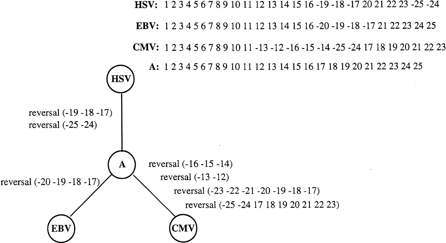
Herpes simplex virus (HSV), Epstein-Barr virus (EBV), and Cytomegalovirus (CMV) gene orders (Hannenhalli et al. 1995) as well as the ancestral gene order (A) and optimal evolutionary scenario recovered by MGR-MEDIAN.
Although the reversal distance for a pair of genomes can be computed in polynomial time (Hannenhalli and Pevzner 1999), its use in studies of multiple genome rearrangements was somewhat limited since it was not clear how to combine pairwise rearrangement scenarios into a multiple rearrangement scenario. In particular, Caprara (1999) demonstrated that even the simplest version of the Multiple Genome Rearrangement Problem, the Median Problem, is NP-hard. As a result this line of research was later abandoned in favor of the breakpoint analysis approach, and the existing tools use the so-called breakpoint distance(Watterson et al. 1982; Nadeau and Taylor 1984) to derive the rearrangement scenarios. However, the breakpoint analysis has some limitations in the analysis of pairwise genome rearrangements (Pevzner 2000). One of the reasons why the breakpoint distance dominated the analysis of multiple rearrangements in the last few years is that it was not clear how to compute the plausible reversal-based evolutionary scenarios. This paper uses the reversal distance for computing multiple rearrangement scenarios and discusses some advantages of this approach over the breakpoint distance approach.
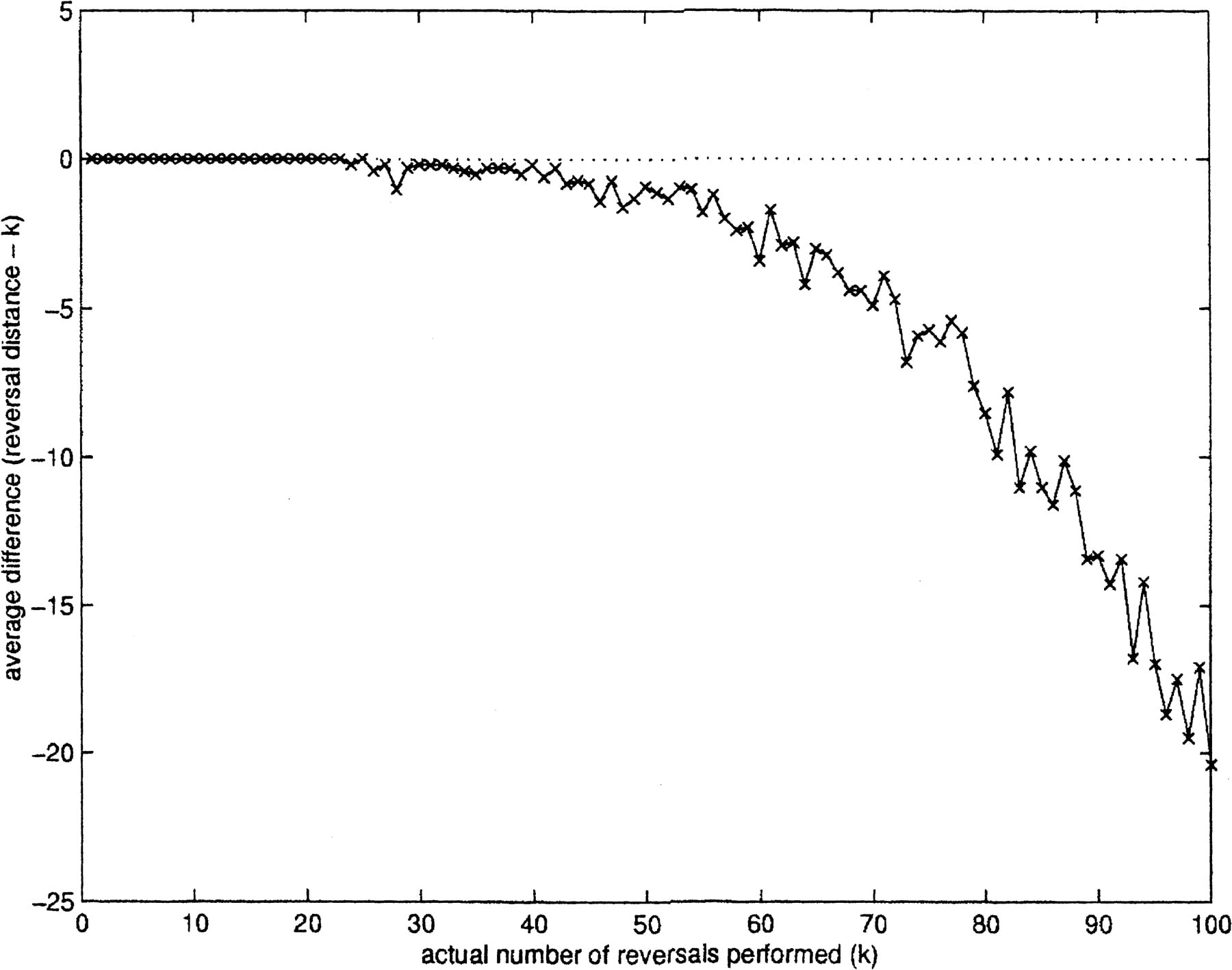
Our algorithm explores the specifics of the reversal distance and is based on the observation that the reversal distance is a good approximation of the true distance for many biologically relevant cases. Let γ be a genome that evolved from a genome π byk reversals (i.e., the true distance between π and γ is k). We say that π and γ form a valid pairif d(π,γ) = k; otherwise we say thatd(π,γ) underestimates the true distance (Wang and Warnow 2001). Typically two genomes form a valid pair if the number of rearrangements between them is relatively small, exactly the case in a number of genome rearrangement studies. Figure1 illustrates that for a genome withn = 100 markers, the reversal distance approximates the true distance very well as long as the number of reversals remains below 0.4n. In many biologically relevant cases (e.g., rearrangements of the X chromosome in mammalian species), the number of rearrangement events is well below 0.4n. As a result, the reversal distance often corresponds to valid (or “almost valid”) pairs of genomes. Therefore the genome-based evolutionary trees are often additive or “almost additive” (Buneman 1971). This property allows one to design new genome rearrangement algorithms that explore the specifics of additive trees.
Reversal distance, d(πγ), versus actual number of reversals performed to transform π into γ, where γ is a genome/permutation that evolved from the identity permutation π = 1,2, … ,100 by k random reversals. The simulations were repeated 10 times for every k. We compute the average difference between the reversal distance and the actual number of reversals performed (k).
Let π and γ be the leaves (existing genomes) in the evolutionary tree T and let π = ς1,ς2, … ,ς k−1,ς k = γ be a path between π and γ in T passing through the ancestral genomes ς2, … ,ς k−1. Define
The paper is organized as follows. In the next section, we review previous work on the Multiple Genome Rearrangement Problem. We then describe a new algorithm to solve the Multiple Genome Rearrangement Problem for unichromosomal genomes. Lastly, we study rearrangements of multichromosomal genomes.
Previous Work
Studies of the Multiple Genome Rearrangement Problem started from the special case of the Median Problem. That is, given the gene order of three unichromosomal genomes G 1,G 2, and G 3, find the ancestral genome A which minimizes the total reversal distanced(A, G 1) + d(A, G 2) + d(A, G 3). Thebreakpoint analysis (Blanchette et al. 1997; Sankoff and Blanchette 1997) attempts to solve the Median Problem by minimizing thebreakpoint distance instead of the reversal distance. A pair of elements in permutations π and γ form a breakpointif they are consecutive in one permutation but nonconsecutive in the other. The breakpoint distance between two permutations is simply the number of breakpoints. Blanchette et al. (1997) and Sankoff and Blanchette (1997) generalized this notion for the case of more than two genomes.
The drawback of breakpoint analysis is that the breakpoint distance, in contrast to the reversal distance, does not correspond to a minimum number of rearrangement events. As a result, the breakpoint median, recovered by breakpoint analysis, rarely corresponds to theancestral median, the genome that minimizes the overall number of rearrangements in the evolutionary scenario. Our simulations demonstrate that in many cases the ancestral median correctly reconstructs the ancestral genome. Another problem with breakpoint analysis is that it is not clear how to adapt it to multichromosomal genomes.
To illustrate the drawbacks of the breakpoint analysis, consider the following simple example. Suppose that the genomesG 1, G 2, and G 3evolved from the ancestral genome A = 1 2 3 4 5 6 by one reversal each such that
This paper studies the ancestral median problem because it appears to be more biologically accurate than the breakpoint median. Initial attempts to recover the ancestral median were made by Hannenhalli et al. (1995) and Sankoff et al. (1996), who came up with approaches that may work well for three close genomes. However, it is not clear how to generalize their approaches for more than three genomes. In particular,Hannenhalli et al. (1995) were successful in reconstructing a genome rearrangement scenario for three herpesviruses but failed to resolve a very complicated dataset of 13 Campanulaceae cpDNAs with 105 markers (the comparative maps were constructed by Mary Beth Cosner and colleagues in the early 1990s). The variety of rearrangements in these flowering plants far exceeds that reported in any group of land plants, thus making this dataset a challenging problem for any genome rearrangement study.
The first relatively large dataset of rearranged genomes was studied byBlanchette et al. (1999), who used BPAnalysis, the original implementation of breakpoint analysis (Blanchette et al. 1997), to analyze 11 metazoan mtDNA with 35 markers. As for theCampanulaceae problem, it remained unsolved for almost ten years until Cosner et al (2000a,b) improved on BPAnalysis and constructed a rearrangement scenario with 67 reversals. Recently, Moret et al. (2001) developed the software GRAPPA, which further improved on BPAnalysis. Finally, in a recent breakthrough, Moret et al. (2001)described a million-fold speedup over GRAPPA and reevaluated theCampanulaceae rearrangement scenario. Their analysis returned 216 trees with reversal distance 67, compared to only four such trees in the previous analysis. Our MGR algorithm described below improves on this recent result by generating a rearrangement scenario with only 65 reversals that was overlooked by Moret et al. (2001).
Multiple Genome Rearrangement Problem
Algorithm
We first explain the idea of our algorithm for the case of three genomes. Our algorithm evaluates all possible reversals for each of the three genomes, identifying good reversals. Intuitively, a reversal is good if it brings a genome closer to the ancestral genome. Of course, the ancestral genome is unknown and therefore it is unclear how to find good reversals. However, we argue (and confirm by simulations) that the reversals which bring G 1closer to both G 2 and G 3 are likely to be good reversals. If this is correct, then we don't need the ancestral genome to find good reversals. We then carry on good reversals in the genomes G 1, G 2, and G 3 in the hope that they will bring us closer to the ancestor, and iterate until the genomes G 1,G 2, and G 3 are transformed into an identical genome (converge to the ancestor A). Ideally, at this point, we have reached the most likely ancestral median. Of course, this approach works well only for “almost additive” trees with small deficit, and we argue that it is the case for many biologically interesting samples.
A good reversal ρ in genome G 1 is a reversal that reduces the reversal distance betweenG 1 and G 2 and the reversal distance between G 1 andG 3. Define Δ(ρ) as the overall reduction in the reversal distances:
The idea of our algorithm is embarrassingly simple: look for good reversals in G 1, G 2, andG 3 and perform them (if there are any) until each of the genomes is turned into the same ancestral genome. In many cases (in particular for additive trees), good reversals are sufficient to bring all three genomes to the ancestor. We call an instance of the median problem that can be resolved using only good reversals a perfect triple. If we run out of good reversals before the three genomes converge to the ancestor, we relax our definition of good reversals.
This approach leaves room for some flexibility. Often there is a variety of good reversals and it is not clear which one to choose. For example, the list of good reversals often contain nonoverlapping reversals ρ(i 1,j 1) and ρ(i 2,j 2) withi 1 ≤ j 1 <i 2 ≤ j 2, and the order in which these reversals are performed is often irrelevant. Our objective is to choose good reversals in such a way that we don't run out of good reversals until all three genomes converge to the ancestor. One way to address this problem is to test all pairs/triples/ … of reversals in order to avoid reversals that would cause us to run out of good reversals in a few steps. We also use a heuristic to choose thebest reversal from the list of good reversals. The heuristic is based on an observation that good reversals, if carried out in the correct order, should not affect most of the other good reversals that are available. Hence, for each good reversal ρ, we computen ρ , the number of good reversals that will be available if ρ is carried out. The heuristic picks the good reversal ρ with the maximal n p as the best reversal, the reversal to be carried out. We implemented these procedures in a program called MGR-MEDIAN, and it turned out to work well in practice.
In some cases, no good reversal will be available; that is, Δ(ρ) < 2 for all reversals ρ in each of the three genomes. In those situations, the best reversal will be the result of a depth k search minimizing the total pairwise reversal distances. Suppose we have a sequence of k reversals ρ1, ρ2 … ρk to be applied to G 1. Define
The depth k search should be taken with caution when one of the genomes is already within distance less than k from the ancestor. In this case we consider k reversals ρ1, ρ2, … ,ρ k , where the firstx reversals are applied to G 1, the nexty reversals are applied to G 2, and the remaining k − x − y reversals are applied to G 3, and maximize the function
In many cases, especially when m is large, we will run out of good reversals before converging to the ancestral genome. In such cases, we have developed a heuristic to complete the recovery of the phylogeny. The heuristic relies on the MGR-MEDIAN program for three genomes described in the previous section. Starting from the three closest genomes (in terms of the reversal distance), it iteratively adds one more genome to reconstruct the full phylogeny. Whenever possible, we choose the genome that is the “closest” to the partially reconstructed tree and such that it also forms a perfect triple with the two endpoints of one of the edges in the tree. We seek the closest genomes first because, as we describe below, the closer the genomes, the more accurate the ancestor produced by MGR-MEDIAN.
Assume that genomes G 1,G 2, … , G l are already included in the tree T that corresponds to the partially reconstructed phylogeny. The problem of adding genomeG l+1 to T corresponds to identifying the edge of T that should be split by the edge leading toG l+1. We call that edge the split edge. The heuristic once again uses a simple greedy approach to find the split edge. For each edge (u, v) in T, computeM = M (u, v, G l+1), the median of u, v, and G l+1. The cost of adding G l+1 to this edge, C(u, v), is the total reversal score of the median less the reversal distance between u and v (the score of the edge being removed). Formally,
The described algorithms rely on our ability to find good reversals. Instead of computing Δ(ρ) for all possible reversals while looking for good reversals, we have implemented a speedup making the algorithms more computationally efficient. The speedup makes use of the concept of conserved adjacency. We call an ordered pair of markers, (x, y), a conserved adjacency if (x, y) or its inverse (−y, −x) is present in all genomes as consecutive elements. When looking for good reversals, we only consider reversals that do not break any conserved adjacency. The justification behind this shortcut comes from a result of Hannenhalli and Pevzner (1996) and a theorem recently proved by Glenn Tesler (pers. comm.).
Tests
Simulated Data
We compared our MGR algorithm to the two implementations of breakpoint analysis: BPAnalysis (Blanchette et al. 1997) and GRAPPA (Moret et al. 2001). Our initial tests showed that these two programs were producing nearly identical results, and so we decided to include only results from GRAPPA, because it was a more efficient implementation. When testing the algorithm, we are interested not only in the phylogeny that we recover but also in the correct labeling of the internal (ancestral) nodes.
We used the following simulated data for benchmarking. Starting from the identity permutation A with n genes/markers, we performed k reversals to get genome G 1,k to get G 2, and k to getG 3. We used the resulting three permutations as the input to MGR-MEDIAN and GRAPPA and checked whether they reconstructed the ancestral identity permutation.
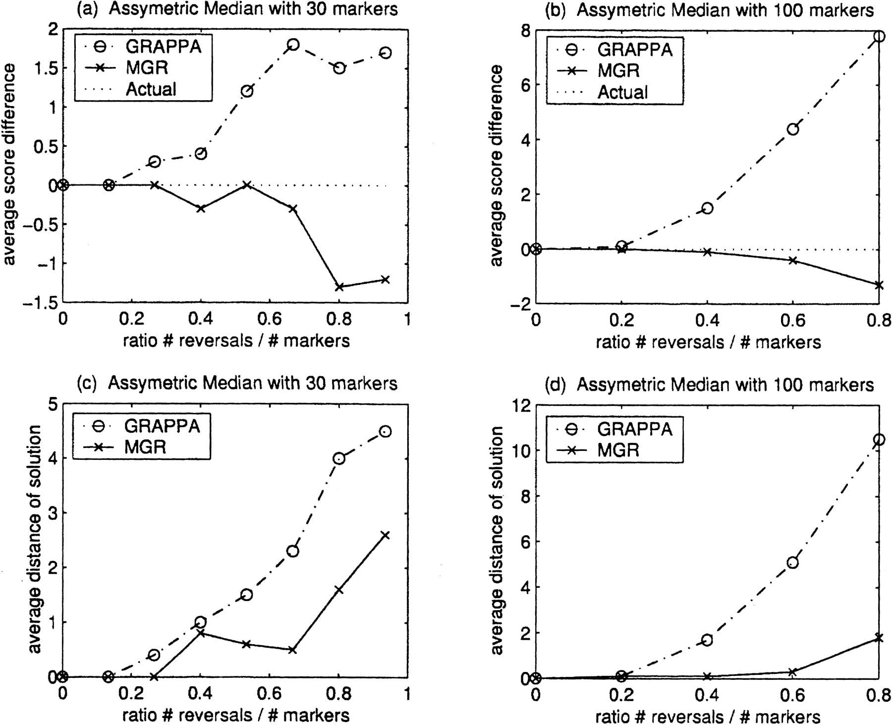
Figure 2a,b shows the difference between the total reversal distance D(T) of the tree recovered by the algorithm and the actual number of reversals (equal to 3k). Figure 2c,d shows the reversal distance between the ancestral permutation recovered by the algorithm and the actual ancestor, the identity permutation. The tests are conducted for various ratios r = #reversals/#markers.
Comparison of MGR-MEDIAN and GRAPPA (three genomes equidistant from the ancestor). The genomes G 1, G 2,G 3 are obtained by k reversals each from the ancestral identity permutation 1 2 … n (n= 30 and n = 100). The simulations were repeated 10 times for every ratio #reversals/#markers = 3k/n. (a) and (b) show the average difference between the number of reversals on the tree recovered by the algorithm and the number of reversals on the actual tree (equal to 3k). (c) and (d) show the average reversal distance between the solution recovered and the actual ancestor.
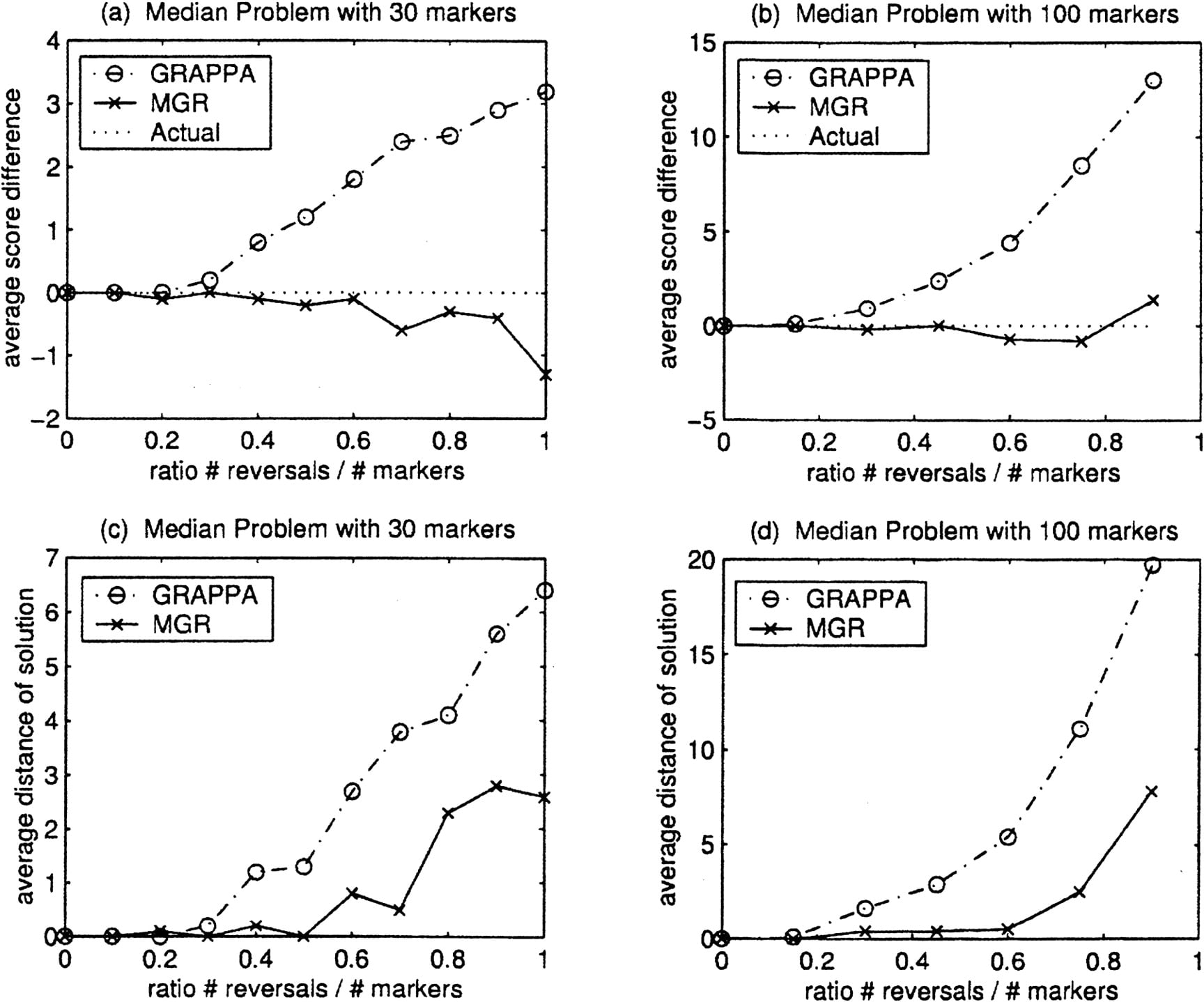
Both GRAPPA and MGR-MEDIAN produce very similar solutions forr < 0.20. But as the ratio r increases, GRAPPA starts making errors. In contrast, MGR-MEDIAN persists in finding correct solutions and in some cases find solutions that even have fewer reversals than the actual ancestor. The issue here is that as the ratior increases, the assumption that the ancestor corresponds to the most parsimonious scenario sometimes fails. In Figure 2c,d we see that as the ratio r increases, both algorithms start having difficulty recovering the actual ancestor, with the solution produced by GRAPPA further away on average than the ancestor produced by MGR-MEDIAN.
Figure 3 presents the results of similar experiments with nonequidistant genomes starting from the identity permutation A and performing k, k, and 2krandom reversals to obtain G 1,G 2, and G 3. Once again, GRAPPA starts failing to recover the optimal solution at r > 0.20, while MGR-MEDIAN keeps finding the true ancestor.
Comparison of MGR-MEDIAN and GRAPPA (three genomes nonequidistant from the ancestor). The genomes G 1,G 2, and G 3 are obtained byk, k, and 2k reversals, respectively, each from the ancestral identity permutation 1 2 … n (n= 30 and n = 100). The simulations were repeated 10 times for every ratio #reversals/#markers = 4k/n. (a) and (b) show the average difference between the number of reversals on the tree recovered by the algorithm and the number of reversals on the actual tree (equal to 4k). (c) and (d) show the average reversal distance between the solution recovered and the actual ancestor.
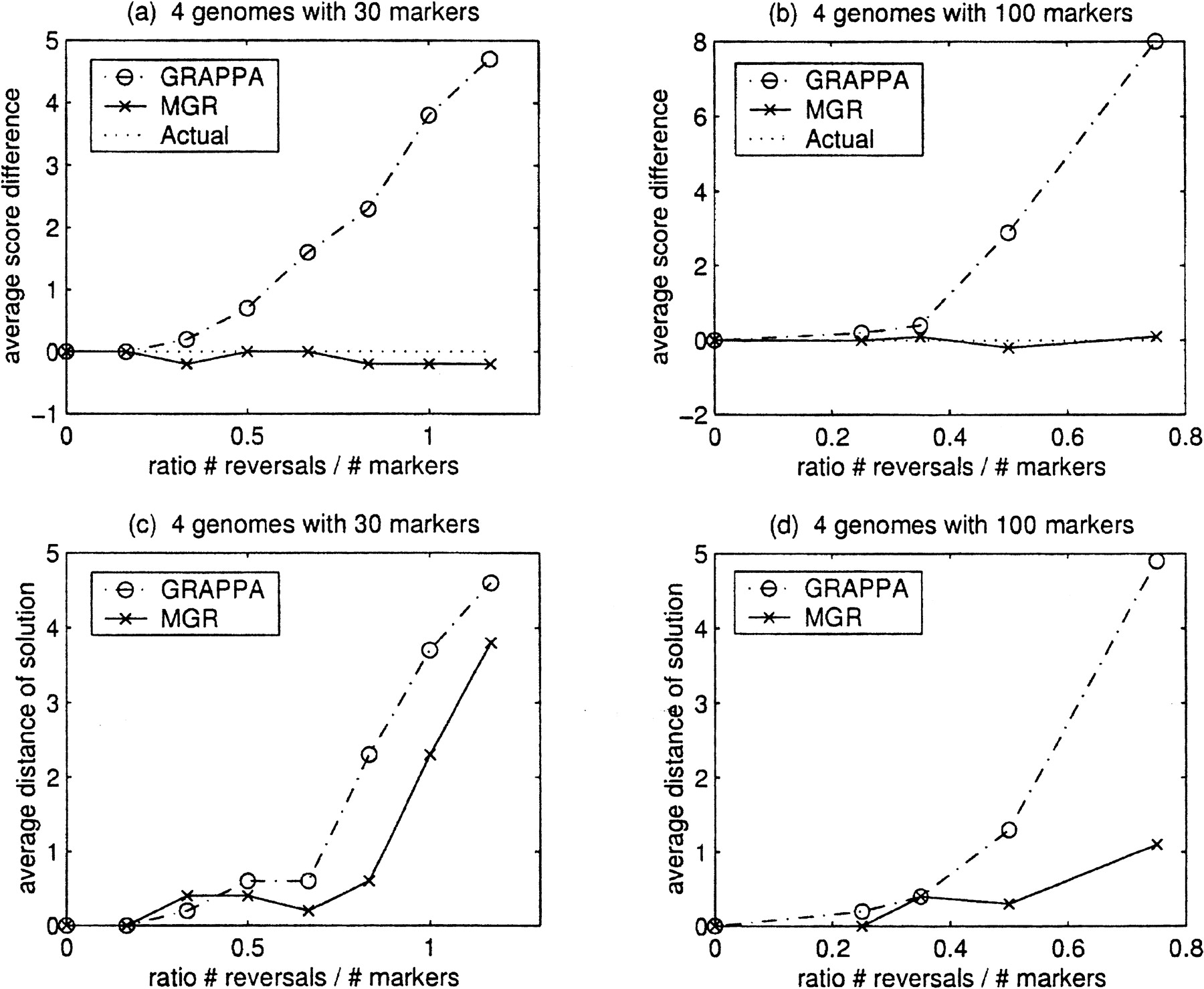
We tested the performance of MGR for four and more genomes using a similar setup. First, we considered a small tree with four genomes as leaves and two internal (ancestral) nodes. For simplicity, we picked one of the ancestral nodes to be the identity permutation. We then randomly simulated k reversals on each branch of the tree. We used the resulting four leaves of the tree as the input for MGR and GRAPPA and calculated the difference between the total reversal distance of the tree recovered with the actual number of performed reversals equal to 5k (Fig. 4a,b). We also calculated how close the solutions recovered would get of the true ancestral permutation (the identity permutation). Since in each solution there are two internal nodes, we picked the one that is closer to the identity and recorded the reversal distance between it and the identity permutation (Fig. 4c,d).
Comparison of MGR and GRAPPA (four genomes). We start from an unrooted tree with four leaves and select one of the two internal nodes to be the identity permutation 1 2 … n (n = 30 and n = 100). We then perform k reversals on each branch of the tree to obtain the genomes G 1,G 2, G 3, and G 4as the four leaves of the tree. The simulations were repeated 10 times for every ratio #reversals/#markers = 5k/n. (a) and (b) show the average difference between the number of reversals on the tree recovered by the algorithm and the number of reversals on the actual tree (equal to 5k). (c) and (d) show the average reversal distance between the best (i.e., closest) internal node in the solution recovered and the identity permutation.
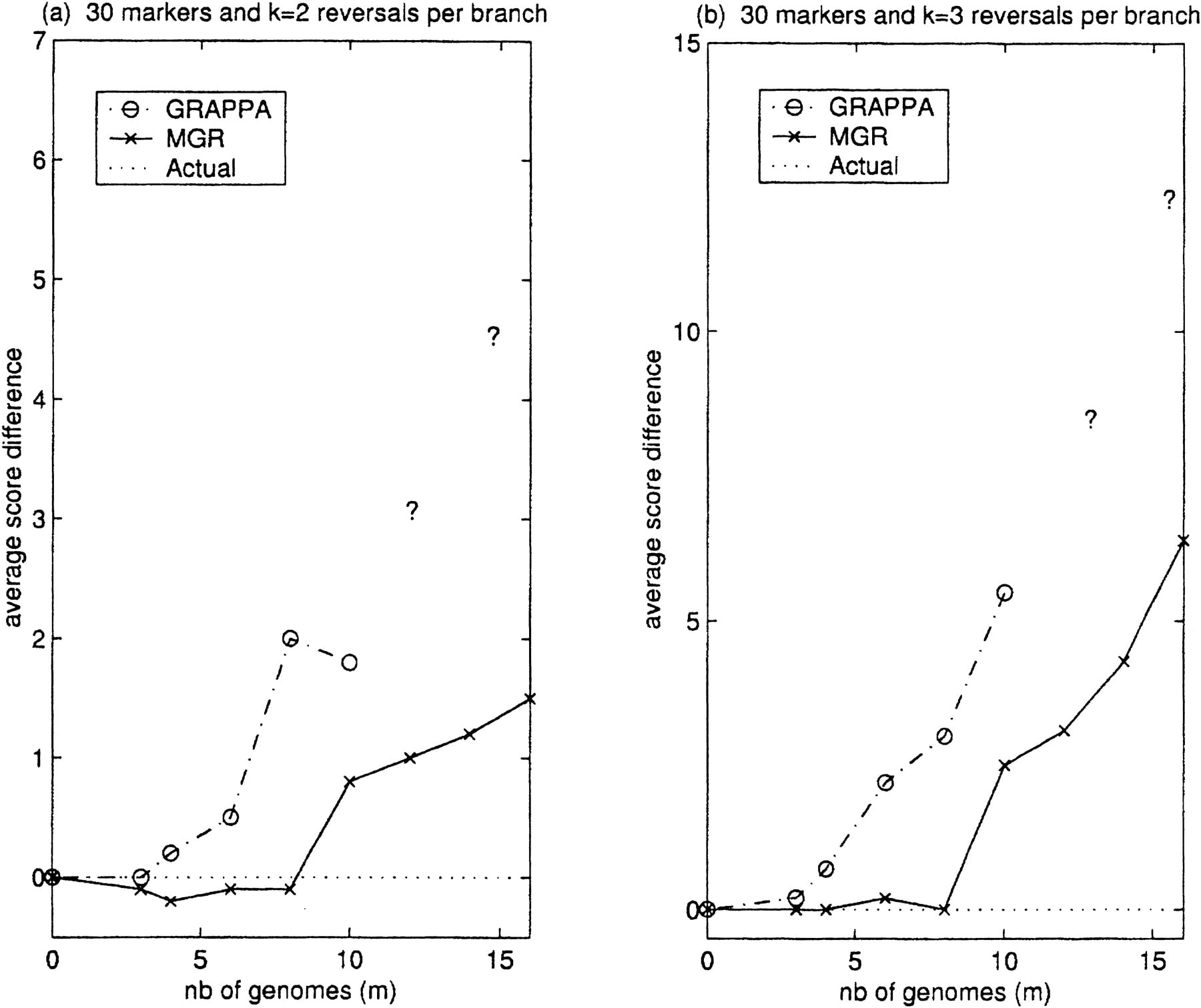
Finally, to see the effect of adding more genomes, we constructed larger complete unrooted binary trees and simulated k random reversals on each branch. To obtain a sample input with mgenomes that we would feed into MGR and GRAPPA, we simulated the smallest complete binary tree such that the number of leaves was larger than m and randomly removed the extra leaves. The results in Figure 5 show the difference between the total reversal distance of the tree recovered and the total reversal distance of the simulated tree. Note that it is difficult to use the ratio r = #reversals/#markers here as it changes depending on the size of the tree. For example, when k = 1, ifm is 4 then r = 5/30 ≈ 0.167, but if mis 8 then r = 13/30 ≈ 0.433, and if m is 16 then r = 27/30 = 0.9. Unfortunately, running GRAPPA on more than 10 genomes turned out to be impossible on our workstations, as the tree space was too large. The only way to get around this problem would have been to suggest a tree topology to GRAPPA (which is exactly what we are trying to recover in the first place). However, even if we did suggest the actual tree topology to GRAPPA, we would still get an average score difference of 7.3 for n = 30 and of 19.1 for n = 100.
Comparison of MGR and GRAPPA (m genomes each with 30 markers). The genomesG 1,G 2, … ,G m correspond to a subset of leaves from a complete unrooted binary tree on which we have performed k reversals on each branch. The simulations were repeated 10 times for every m. (a) and (b) show the average difference between the number of reversals on the tree recovered by the algorithm and the number of reversals on the actual tree when k = 2 and k = 3, respectively.
Herpesvirus Data
Hannenhalli et al. (1995) used herpesvirus gene orders as a test case for one of the first studies on the Multiple Genome Rearrangement Problem. They developed a rather elaborate method to solve a relatively simple instance of the median problem for Herpes simplex virus (HSV), Epstein-Barr virus (EBV), and Cytomegalovirus (CMV) (Fig. 6a). As the authors themselves pointed out, the method used would not be applicable to more complex problems and new algorithms would be required. The optimal solutions recovered involved seven reversals. The ratio of #reversals/#markers in this example is: r = 7/25 = 0.28. Our simulations indicate that MGR-MEDIAN typically reconstructs the correct scenario with such ratios, whereas GRAPPA typically fails forr > 0.2.
We tested both MGR-MEDIAN and GRAPPA on these three herpesviruses to see whether they would recover the ancestral genome suggested byHannehalli et al. (1995). MGR-MEDIAN found this genome and reconstructed the rearrangement scenario with seven reversals (Fig. 6b) even though it did not correspond to a perfect triple. In contrast, GRAPPA returned a suboptimal solution with eight reversals. Actually, the ancestor suggested by GRAPPA was the genome HSV itself, indicating the problem with the breakpoint distance described earlier.
Human, Fruit Fly, and Sea Urchin mtDNA Data
Sankoff et al. (1996) analyzed human, sea urchin, and fruit fly mtDNA to derive the ancestral gene order. Using MGR-MEDIAN, we found the ancestral gene order A with a total reversal distance of 39 (Fig. 7). The solution is different from the ones found by Sankoff et al., but the total reversal distance is the same. The ratio of #reversals/#markers for this data set isr = 39/33 ≈ 1.18, an indication of a difficult problem. Running GRAPPA on these genomes, we obtained a solution that has a total reversal distance of 43.
Human, sea urchin, and fruit fly mitochondrial gene order taken fromSankoff et al. (1996). A is the ancestral gene order suggested by MGR-MEDIAN.

Metazoan mtDNA Data
Blanchette et al. (1999) used BPAnalysis in the rearrangement study of 11 metazoan mtDNAs. The genomes come from six major metazoan groupings: nematodes (NEM), annelids (ANN), mollusks (MOL), arthropods (ART), echinoderms (ECH), and chordates (CHO). They were originally selected by those authors to provide the analysis with exemplar of the most diverse members of each group. The two “optimal” phylogenies recovered in their study had 199 breakpoints.
We studied the same dataset with MGR and GRAPPA and used the curated gene order data of the 11 genomes from the MGA Source Guide compiled by Jeffrey L. Boorehttp://www.jgi.doe.gov/programs/comparative/MGA_Source_Guide.html. After removing two genes that were not shared by all mtDNA, we were left with a common set of 36 genes. MGR recovered a phylogeny with 150 reversals (Fig. 8). The tree space for 11 genomes is very large, and searching it exhaustively with GRAPPA is very time consuming. After 48 hours on a workstation, GRAPPA had recovered three “optimal” trees with 175 reversals and 200 breakpoints. Even suggesting the topology found by MGR to GRAPPA would only produce a fourth tree with 175 reversals.
Phylogeny of 11 metazoan genomes reconstructed by MGR. The gene order data is taken from the MGA Source Guide compiled by Jeffrey L. Boore. The genomes come from 6 major metazoan groupings: nematodes (NEM), annelids (ANN), mollusks (MOL), arthropods (ART), echinoderms (ECH), and chordates (CHO). Numbers show the number of reversals.
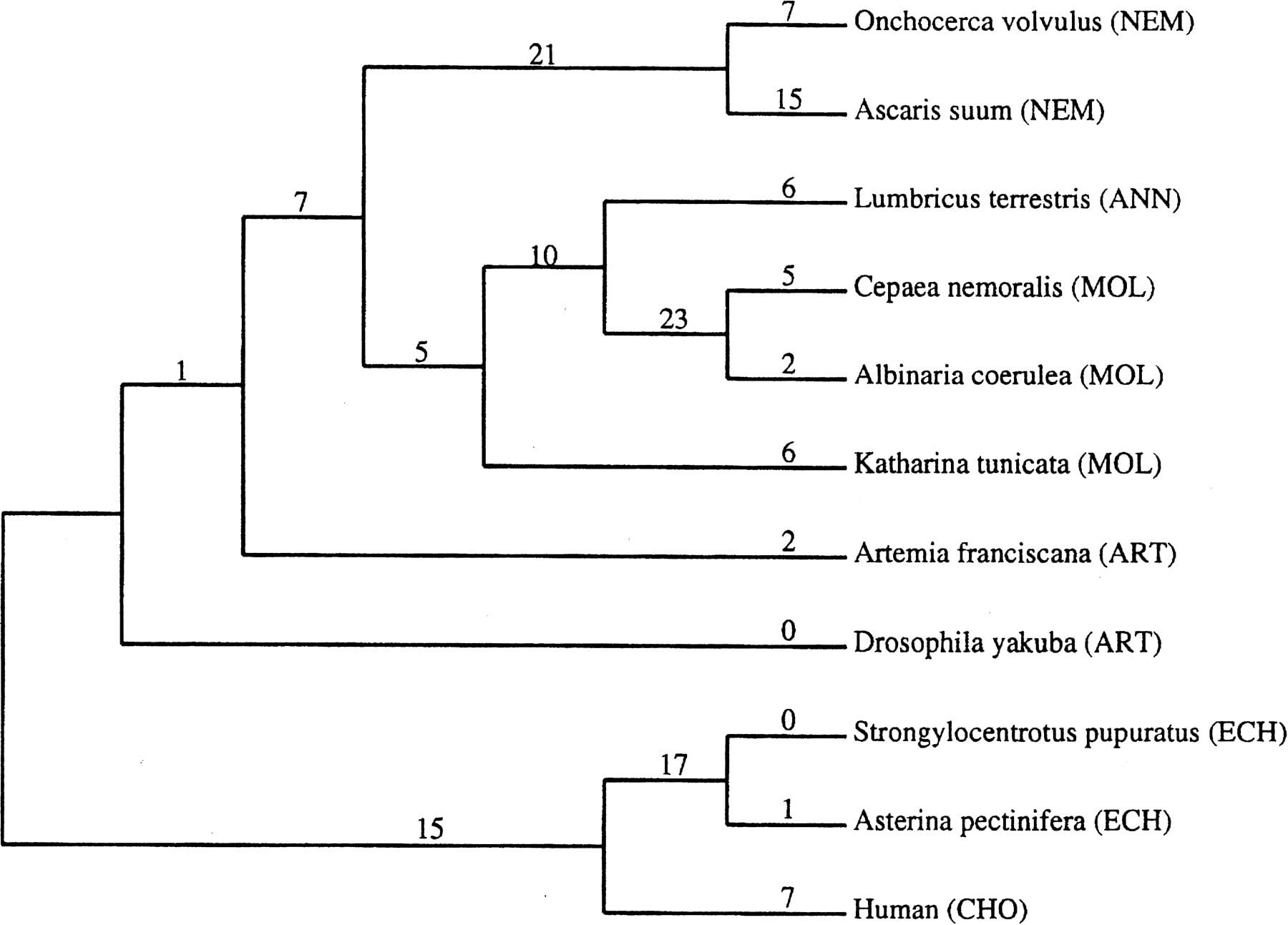
The tree recovered by MGR is closely related to one of the optimal trees described in the study by Blanchette et al. (1999). The weak association of Katharina tunicata with the mollusks was already discussed by those authors. Apart from this and from the weak grouping of the two arthropods, the induced phylogeny also agrees with the metazoan phylogeny proposed by Boore and Brown (2000); the nematodes and echinoderms were not discussed in that paper. We note that Blanchette et al. (1999) obtained their tree in a semiautomated regime by making a selection between the potential phylogenies and disregarding the ones breaking any one of the six metazoan groupings. Although such assumptions about the data were not included in MGR, it did not prevent it from the discovery of a very similar tree in a fully automated fashion (Fig. 8). Rooted differently, we see that the nematodes are a late-branching sister taxon of the annelids which is the same as in Blanchette et al. (1999). The deuterostomes (chordate and echinoderm) association was successfully identified in bothBlanchette's 1999 study and in the tree from MGR but not in any of the first three trees produced by GRAPPA (excluding the one we suggested as a constraint).
Campanulaceae cpDNA Data
We analyzed the Campanulaceae Chloroplast dataset with 13 cpDNAs and 105 markers. It is one of the most challenging genome rearrangement datasets studied by Cosner et al. (2000a,b) and Moret et al. (2001). The tree space for 13 genomes is too large and cannot be searched exhaustively by GRAPPA. To analyze the tree space in this case, those two groups of authors described various techniques to obtain constraint trees to suggest to the program. GRAPPA then searched the space of refinements of these constraint trees trying to minimize the total number of reversals. Moret et al. (2001) recovered 216 trees with a total of 67 reversals. GRAPPA was not able to decide which of those trees corresponds to the most likely reconstruction of the rearrangement scenario.
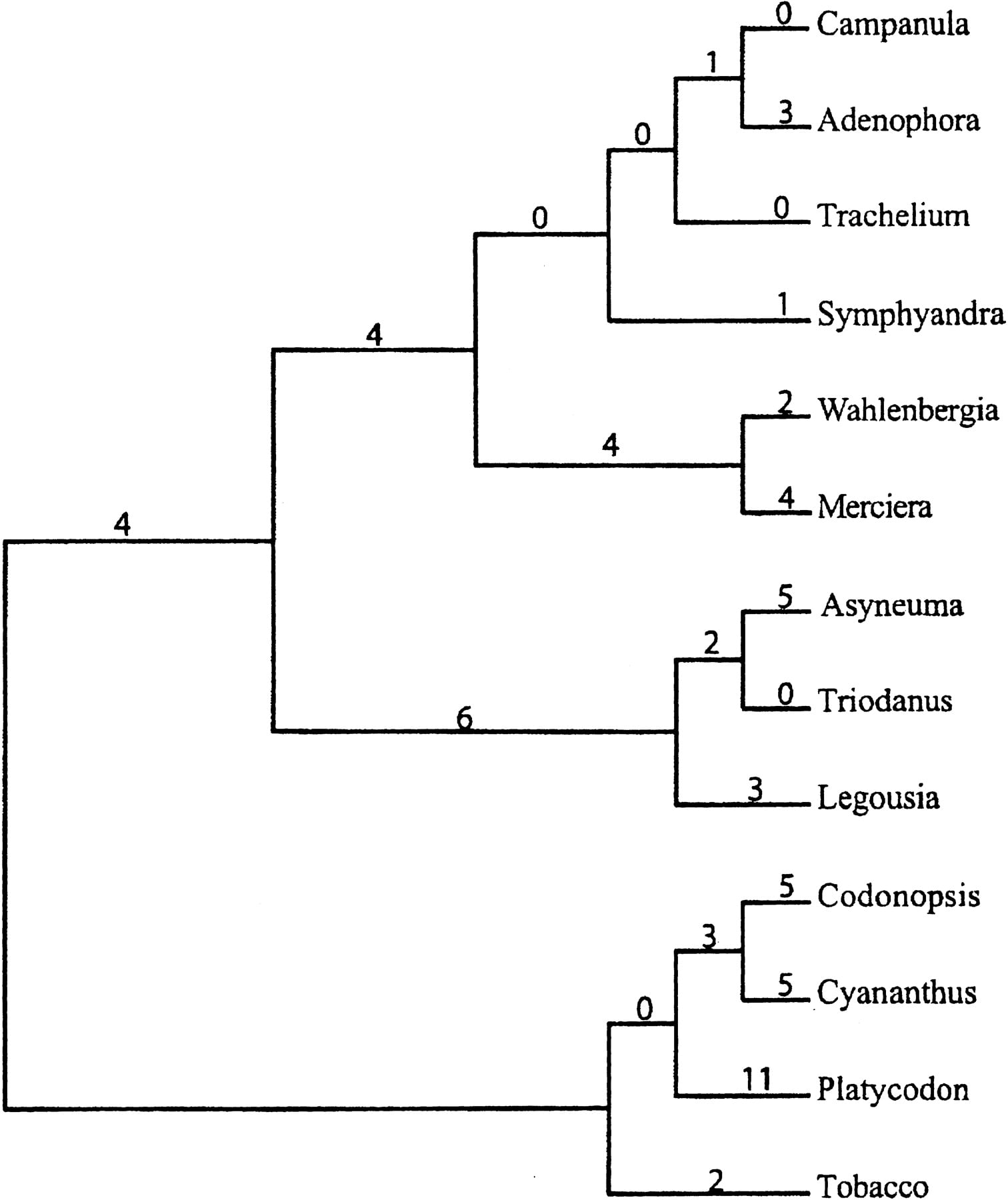
Running MGR on the same data set did not require the preprocessing of a constraint tree and recovered a tree with only 65 reversals, shown in Figure 9. The topology of the tree recovered actually corresponds to the topology of one of the trees recovered by GRAPPA, but the labeling of the internal nodes differs. Because our tree minimizes the number of reversals, we argue that MGR provided a better reconstruction of the rearrangement scenario compared to GRAPPA.
Phylogeny of the Campanulaceae cpDNA dataset as reconstructed by MGR. Numbers show the number of reversals.
Reconstructing Ancestral Gene Orders for Multichromosomal Genomes
Algorithm
Consider three multichromosomal genomes G 1,G 2, and G 3. The median problem is to find the ancestral genome A which minimizes the totalgenome distance d(A,G 1) +d(A,G 2) +d(A,G 3). The genomic distance in this case is defined in terms of reversals, translocations, fusions, and fissions, the most most common rearrangement events in multichromosomal genomes (Pevzner 2000).
Let π = π1 … π n be a chromosome in a multichromosomal genome and 1 ≤ i ≤j ≤ n. A reversal ρ(π,i,j) rearranges the genes inside π and transforms it into π1 … π i−1 − π j − π j−1 … − π i π j+1 … π n . Let π = π1 … π n and ς = ς1 … ς m be two different chromosomes and 1 ≤ i ≤ n + 1 and 1 ≤j ≤ m + 1. A translocationρ(π,ς,i,j) exchanges genes betweenchromosomes π and ς and transforms them into chromosomes π1 … π i−1ς j … ς m and ς1 … ς j−1π i … π n . A fusion concatenates the chromosomes π and ς, resulting in a chromosome π1 … π n ς1 … ς m . A fission “breaks” a chromosome π into two chromosomes, π1 … π i−1 and π i … π n .
Given two genomes Π and Γ, the genomic distance, d(Π,Γ), is defined as the minimum number of reversals, translocations, fusions, and fissions required to convert one genome into the other. The genomic distance was first studied by Hannenhalli and Pevzner (1995), who developed a polynomial-time algorithm to compute a rearrangement scenario between human and mouse involving 131 rearrangements.
The MGR-MC algorithm is a generalization of the MGR-MEDIAN algorithm for unichromosomal genomes. First, we evaluate all possible rearrangements (reversals, translocations, fusions, and fissions) for each of the three genomes, identifying good rearrangements. As in the section on Tests above, a rearrangement is good if it brings a genome closer to the ancestral genome. We will argue once again that the rearrangements which bring G 1 closer toboth G 2 and G 3 are likely to be good. We iteratively carry on these good rearrangements until the genomes G 1, G 2, andG 3 are transformed into an identical genome, hoping that we have reached the most likely ancestral median.
Since we are dealing with multichromosomal genomes and with four different types of rearrangements, we need to be aware of an ambiguous situation that can occur when solving the median problem. Consider the following simple example:
Tests
Simulated Data
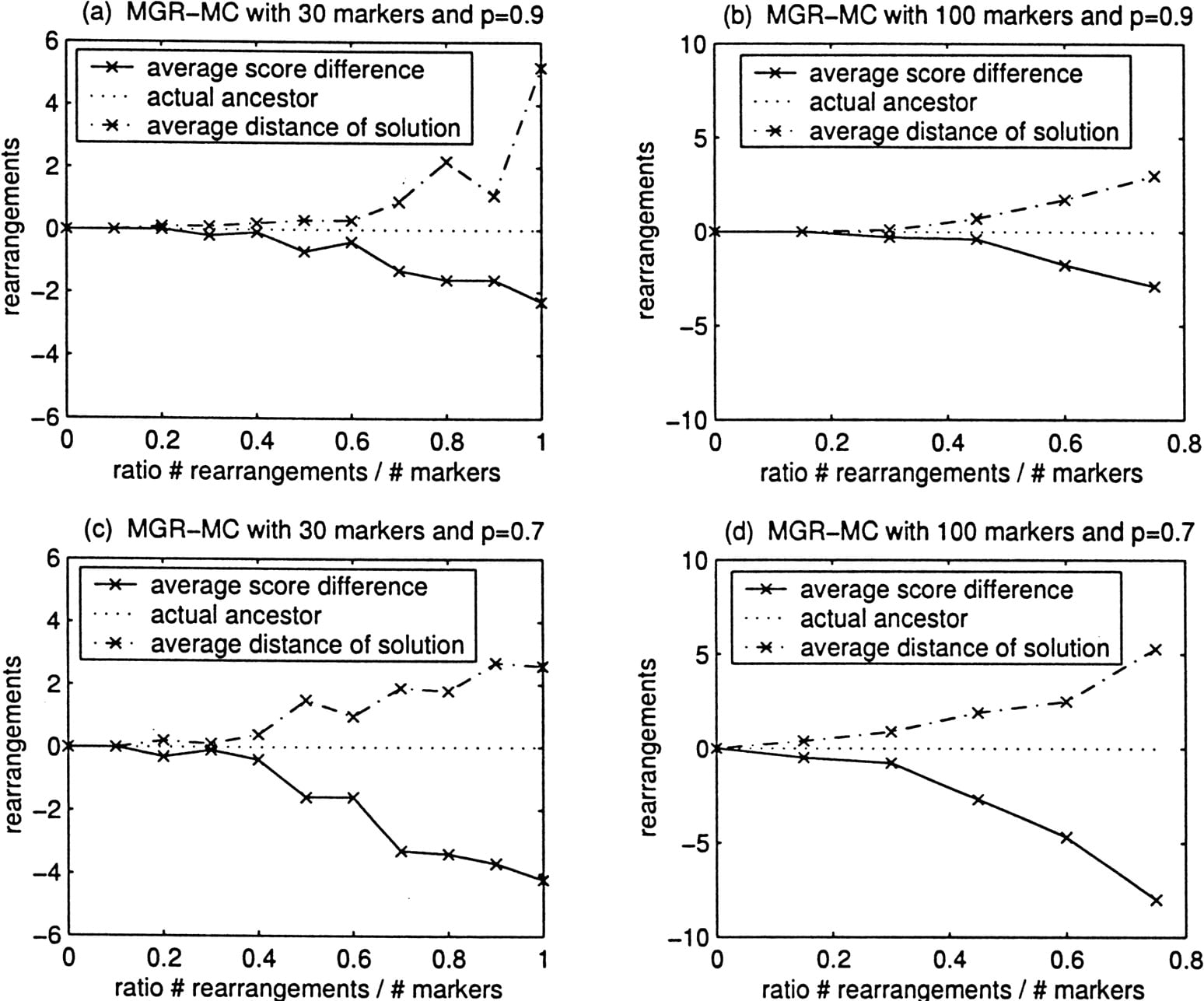
We used the following simulations to test the performance of MGR-MC. Starting from the identity permutation A of size n,we first randomly selected b chromosome breaks to simulate a multichromosomal ancestor. Next, to transform A intoG i (1 ≤ i ≤ 3), we performedk rearrangements where each rearrangement was randomly assigned to be a reversal/translocation with probability p and a fusion/fission with probability 1 − p. We used the resulting three genomes as the input for MGR-MC. We are interested in the difference between the score (total number of rearrangements) of the solution recovered by the algorithm and the actual score of the simulated tree (equal to 3k). We are also interested in the rearrangement distance between the ancestral genome recovered by the algorithm and the actual ancestor. The tests are conducted for various ratios of r = #rearrangements/#markers.
Figure 10 illustrates that MGR-MC has no difficulty recovering ancestral genomes with a score which is at least as good as the one of the actual ancestor. Actually, in all the tests conducted, not once was the solution produced by MGR-MC worse than the true ancestor. The solutions produced for small ratios r = #rearrangements/#markers tend to be very close to the actual ancestor. But, as the ratio r increases, we see the same effect as for unichromosomal genomes: MGR-MC starts finding solutions with a genomic distance which is smaller than the true number of rearrangement events. As a result, the average distance between the solution recovered and the true ancestor increases. The comparison of Figure 10a–d illustrates that the accuracy of reconstructions deteriorates with the increase in the rate of fusions/fissions.
Performance of MGR-MC (three multichromosomal genomes equidistant from the ancestor). The ancestral genomes are obtained from the identity permutation 1 2 … n (n = 30 and n= 100) by inserting b chromosomes breaks (b = 2 when n = 30 and b = 9 when n = 100). The genomes G 1, G 2, andG 3 are obtained by k rearrangements each from the ancestral genomes. Each rearrangement is a reversal/translocation with probability p and a fusion/fission with probability 1 − p. The simulations were repeated 10 times for every ratio #rearrangements/#markers = 3k/n. We compute the average score difference, which is the difference between the number of rearrangements on the tree recovered by the algorithm and the actual number of rearrangements (equal to 3k). We also compute theaverage distance of solution between the solution recovered and the actual ancestor.
Gene Order of the Human-Cat-Mouse Common Ancestor
The modern comparative mapping studies generated a wealth of data on differences in genomic organization for many mammalian species. However, most existing comparative maps are pairwise maps representing genome organization of two species rather thanmultiple maps representing the genomic organization for more than two species. Since the number of established universalmarkers (O'Brien et al. 1999) that work across many genomes is relatively small, it is often not clear how to integrate pairwise comparative maps into multiple maps. The first sufficiently detailed triple comparative maps appeared recently as the results of rat (Watanabe et al. 1999) and cat (Murphy et al. 2000) comparative mapping projects. We collaborated with Bill Murphy to integrate the pairwise human-mouse, human-cat, and mouse-cat comparative maps into a triple human-mouse-cat map, and we use this map for deriving the ancestral genome organization.
The previous attempts to derive rearrangement history of multichromosomal genomes concentrated on human and mouse genomes (Nadeau and Taylor 1984; Hannenhalli and Pevzner 1995). The cat data used in this paper comes from Murphy et al. (2000) and consists of 193 markers shared by all three species. The number of markers is still too small to derive a detailed rearrangement scenario, but it allows one to get some insights into a large-scale organization of the ancestor. Ultimately, this organization may be refined with MGR-MC as soon as more markers shared by all three species become available.
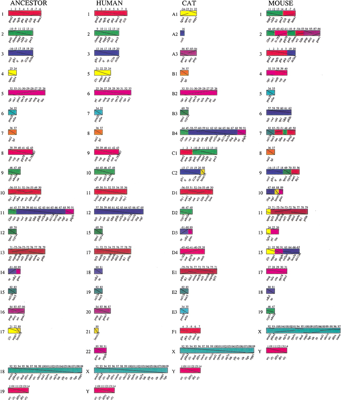
Comparative maps usually correspond to unsigned permutations; that is, no information on the direction (signs) of the genes/markers is available. Since mammalian comparative maps contain manysingletons (Pevzner 2000) the existing algorithms for analyzing unsigned permutations become too time-consuming in this case. As a result, we have to assign an orientation to the markers, since the current implementation of MGR-MC only supports signed permutations/genomes. Ultimately, this should not be a problem as more data become available. We used strips in unsigned permutations (Hannenhalli and Pevzner 1996) to infer the signed permutations from the original unsigned permutations. Using the human genome as a reference, we first identified all the strips in both the cat and mouse genomes. We then assigned an orientation to the markers based on these strips. Any marker for which we could not assign an orientation using this method in either the cat or mouse genome was removed, and we were left with a common set of 114 markers. This process obviously inserts a bias towards blocks of preserved markers, while removing information about more local disruptions, for example, single marker reversals. The resulting ancestral gene order generated by MGR-MC is shown in Figure11. Although most of the elements of the ancestral organization in Figure 11 are consistent with the existing biological conjectures, the organization of ancestral chromosomes 4 and 17 is surprising and even counterintuitive. According to our scenario, the chromosomes 4 and 17 in the ancestor were combined into chromosome 5 in human and chromosome A1 in cat. We do not argue that it is a correct reconstruction of the ancestral chromosomes 4 and 17 (more markers are needed to support this conjecture) but remark instead that MGR-MC provided us with solid combinatorial reasons why such a scenario makes sense. Such reasons are not straightforward and are hard to explain without the multichromosomal genome rearrangement software that was not available to evolutionary biologists in the past. Therefore, the non-trivial combinatorial arguments used by MGR-MC in the construction of Figure 11 may have escaped the attention of biologists who studied this problem in the past. The detailed biological analysis of our human-mouse-cat ancestral reconstruction will be discussed in another paper (joint project with Bill Murphy).
Ancestral median for human, mouse, and cat genomes found by MGR-MC. We used the gene order of 114 markers spread over the chromosomes in all three species. The numbers above the chromosomes correspond to these 114 markers, and the numbering is such that the human genome corresponds to the identity permutation broken into 20 pieces. The names below the chromosomes correspond to the name of the markers. We attribute a color to each human chromosome. The colorof any marker (in any genome) indicates the human chromosome on which the homolog of this marker lies. Each marker segment is traversed by a diagonal line. These diagonal lines are such that the human chromosomes are traversed from top left to bottom right and are designed to provide visual help to identify where rearrangements occurred. For example, for chromosome X, the gene order of the ancestor coincides with the cat gene order and only differs by one segment consisting of genes 108 and 109 (break in the diagonal line) from the human gene order. The mouse X chromosome is broken into 7 segments compared to the ancestor (shown by seven broken segments of the diagonal line).
We thank Bernard Moret and Glenn Tesler for providing their genome rearrangement programs, Bill Murphy for providing us with the cat comparative maps prior to publication and for many helpful discussions, Glenn Tesler for multiple discussions and comments that significantly improved the manuscript, and Tandy Warnow for some useful references. This research is supported by grants from the National Sciences and Engineering Research Council of Canada.
The publication costs of this article were defrayed in part by payment of page charges. This article must therefore be hereby marked “advertisement”; in accordance with 18 USC section 1734 solely to indicate this fact.
Notes
[1] Corresponding author.
Notes
[2] E-MAIL [email protected]; FAX (213) 740-2424
[3] Article and publication are at www.genome.org/cgi/doi/
References
- ↵V. BafnaP. Pevzner(1995) Sorting by reversals: Genome rearrangements in plant organelles and evolutionary history of X chromosome. Mol. Biol. Evol. 12:239–246.
- ↵A. Bergeron(2001) A very elementary presentation of the Hannenhall-Pevzner theory. Proceedings of the Twelfth Annual Symposium on Combinatorial Pattern Matching 2089 of Lecture Notes in Computer Science:106–117, . Jerusalem, Israel. Springer-Verlag, New York..
- ↵P. BermanS. Hannenhalli(1996) Fast sorting by reversal. Combinatorial Pattern Matching. Seventh Annual Symposium 1075, of Lecture Notes in Computer Science, pp. 168–185. Springer, New York..
- ↵M. BlanchetteG. BourqueD. Sankoff(1997) Breakpoint phylogenies. in Genome Informatics Workshop (GIW 1997) eds S. MiyanoT. Takagi(University Academy Press, Tokyo), pp 25–34.
- ↵M. BlanchetteT. KunisawaD. Sankoff(1999) Gene order breakpoint evidence in animal mitochondrial phylogeny. J. Mol. Evol. 49:193–203.
- ↵J. BooreW. Brown(2000) Mitochondrial genomes of galthealinum, helobdella, and platynereis: Sequence and gene arrangement comparisons show that pogonophora is not a phylum and annelida and arthropoda are not sister taxa. Mol. Biol. Evol. 7:87–106.
- ↵P. Buneman(1971) The recovery of trees from measures of dissimilarity. Mathematics in the Archaeological and Historical Sciences (Edinburgh University Press, Edinburgh), pp 387–395.
- ↵A. Caprara(1999) Formulations and complexity of multiple sorting by reversals. in Proceedings of the Third Annual International Conference on Computational Molecular Biology (RECOMB-99) ed S. Istrail(ACM Press, Lyon, France), pp 84–93.
- M. CosnerR. JansenB. MoretL. RaubesonL. WangT. WarnowS. Wyman(2000) An empirical comparison of phylogenetic methods on chloroplast gene order data in campanulaceae. Comparative Genomics (DCAF-2000) (Kluwer Academic Publ. Montreal, Canada), pp 99–121.
- ↵(2000) A new fast heuristic for computing the breakpoint phylogeny and experimental phylogenetic analyses of real and synthetic data. Proceedings of the Eighth International Conference on Intelligent Systems for Molecular Biology (ISMB-2000) (AAAI Press, Menlo Park, California), pp 104–115, ibid.
- ↵T. DobzhanskyA. Sturtevant(1938) Inversions in the chromosomes of Drosophila pseudoobscura. Genetics 23:28–64.
- ↵D. GraurW.-H. Li(2000) Fundamentals of Molecular Evolution. (Sinauer Associates, Sunderland, Massachusetts).
- ↵S. HannenhalliC. ChappeyE. KooninP. Pevzner(1995) Genome sequence comparison and scenarios for gene rearrangements: A test case. Genomics 30:299–311.
- ↵S. HannenhalliP. Pevzner(1995) Transforming cabbage into turnip (polynomial algorithm for sorting signed permutations by reversals). Proceedings of the Twenty-seventh Annual ACM-SIAM Symposium on the Theory of Computing (ACM Press, New York), pp 178–189.
- S. HannenhalliP. Pevzner(1995) Transforming men into mice: Polynomial algorithm for genomic distance problem. Proceedings of the Thirty-Sixth IEEE Symposium on Foundations of Computer Science (IEEE Press, Los Alamtos, California), pp 581–592.
- ↵S. HannenhalliP. Pevzner(1996) To cut… or not to cut (applications of comparative physical maps in molecular evolution). Proceedings of the Seventh ACM-SIAM Symposium on Discrete Algorithms (SODA) (ACM Press, New York), pp 304–313.
- ↵S. HannenhalliP. Pevzner(1999) Transforming cabbage into turnip: Polynomial algorithm for sorting signed permutations by reversals. Journal of Association for Computing Machinery. 46:1–27.
- ↵H. KaplanR. ShamirR. Tarjan(1997) Faster and simpler algorithm for sorting signed permutations by reversals. Proceedings of the Eighth Annual ACM-SIAM Symposium on Discrete Algorithms (ACM Press, New York), pp 344–351.
- ↵J. KececiogluD. Sankoff(1994) Efficient bounds for oriented chromosome inversion distance. in Combinatorial Pattern Matchings. Fifth Annual Symposium, eds M. CrochemoreD. Gusfield(Springer, New York), 807 of Lecture Notes in Computer Science:307–325.
- ↵E.S. LanderL.M. LintonB. BirrenC. NussbaumM.C. ZodyJ. BaldwinK. DevonK. DevarM. DoyleW. Fitzhuge(2001) Initial sequencing and analysis of the human genome. Nature 409:860–921.
- ↵B. MoretL. WangT. WarnowS. Wyman(2001) New approaches for reconstructing phylogenies from gene order data. Proc. Int. Conf. Intell. Syst. Mol. Biol. (ISMB-2001) pp 165–173.
- B. MoretS. WymanD. BaderT. WarnowM. Yan(2001) A new implementation and detailed study of breakpoint analysis. Pac. Symp. Biocomput. (PSB 2001) (AAAI Press, Menlo Park, California), pp 583–594.
- W. MurphyR. StanyonS. O'Brien(2001) Evolution of mammalian genome organization inferred from comparative gene mapping. Genome Biol. 2:1–8.
- ↵W. MurphyS. SunZ.-Q. ChenN. YuhkiD. HirschmannM. Menotti-RaymondS. O'Brien(2000) A radiation hybrid map of the cat genome: Implications for comparative mapping. Genome Res. 10:691–702.
- ↵J. NadeauB. Taylor(1984) Lengths of chromosomal segments conserved since divergence of man and mouse. Proc. Natl. Acad. Sci. 81:814–818.
- ↵S. O'BrienM. Menotti-RaymondW. MurphyW. NashJ. WienbergR. StanyonN. CopelandN. JenkinsJ. WomackJ. Graves(1999) The promise of comparative genomics in mammals. Science 286:458–481.
- ↵R. OlmsteadJ. Palmer(1994) Chloroplast DNA systematics: A review of methods and data analysis. Am. J. Bot. 81:1205–1224.
- ↵J. Palmer(1992) Chloroplast and mitochondrial genome evolution in land plants. in Cell Organelles, ed R. Hermannpp 99–133.
- ↵J. PalmerL. Herbon(1988) Plant mitochondrial DNA evolves rapidly in structure, but slowly in sequence. J. Mol. Evol. 27:87–97.
- ↵P. Pevzner(2000) Computational molecular biology: An algorithmic approach, ch. 10. (MIT Press, Cambridge, Massachusetts).
- ↵D. Sankoff(1992) Edit distance for genome comparison based on non-local operations. in Proceedings of the Third Annual Symposium on Combinatorial Pattern Matching, ed A. Apostolico(Springer-Verlag, Berlin), pp 121–135.
- ↵D. SankoffM. Blanchette(1997) The median problem for breakpoints in comparative genomics. Computing and Combinatorics, Proceedings of COCOON '97, Lecture Notes in Computer Science (Springer-Verlag, New York), pp 251–263.
- ↵D. SankoffG. LeducN. AntoineB. PaquinB. LangR. Cedergren(1992) Gene order comparisons for phylogenetic inference: Evolution of the mitochondrial genome. Proc. Natl. Acad. Sci. 89:6575–6579.
- ↵D. SankoffG. SundaramJ. Kececioglu(1996) Steiner points in the space of genome rearrangements. International Journal of the Foundations of Computer Science 7:1–9.
- ↵Tesler, G. 2002. GRIMM: Genome Rearrangement Web Server.Bioinformatics (in press)..
- ↵J.C. VenterM.D. AdamsE.W. MyersP.W. LiR.J. MuralG.G. SuttonH.O. SmithM. YandellC.A. EvansR.A. Holt(2001) The sequence of the human genome. Science 291:1304–1352.
- ↵Wang, L.-S. and Warnow, T. Estimating true evolutionary distances between genomes. 2001. In: Proceedings of the Thirty-third Symposium on Theory of Computing (STOC'01), pp. 637–646. ACM Press, New York..
- ↵T. WatanabeM. BihoreauL. McCarthyS. KiguwaH. HishigakiA. TsujiY. YamasakiA. Mizoguchi-MiyakitaT. OnoS. Okuno(1999) A radiation hybrid map of the rat genome containing 5,255 markers. Nat. Genet. 22:27–36.
- ↵G. WattersonW. EwensT. HallA. Morgan(1982) The chromosome inversion problem. J. Theor. Biol. 99:1–7.