A Bayesian framework for inferring dynamic intercellular interactions from time-series single-cell data

Overview of DIISCO

DIISCO captures the temporal dynamics and interactions of cell types using scRNA-seq data from multiple time points. We define cell types or states as clusters of cells with similar gene expression profiles in scRNA-seq data. The time-series single-cell data are first merged to define unique cell types or states through typical clustering approaches (Levine et al. 2015; Wolf et al. 2018). The pooling of cells helps with improving statistical power in the detection of rare cell types. Then, the number of cells assigned to each cell type at each time point is computed and used as training data for DIISCO (Fig. 1A). The cell type dynamics can be in the form of cell counts at each time point or standardized proportions of each cell type, that is, normalized by total cells in the sample collected at each time point. Using proportions is often useful in complex patient data where the sampling and quality of biopsies are inconsistent over time points (Maurer et al. 2024).

Figure 1.

Overview of DIISCO framework. (A) General workflow of the DIISCO algorithm including inputs and outputs. Cell type proportions are computed from scRNA-seq data in each time point. Expression of R–L complexes is incorporated to obtain time-resolved interactions between cell types. (B) Network diagram of the model framework. (C) Graphical model of DIISCO, including all hyperparameters. Latent variables are depicted as white circles, and observed variables are depicted as yellow-shaded circles. (D) Process for incorporating domain knowledge on R–L interactions as a prior for cell–cell interactions into DIISCO.

Open in new tabDownload PowerPointLink to figure

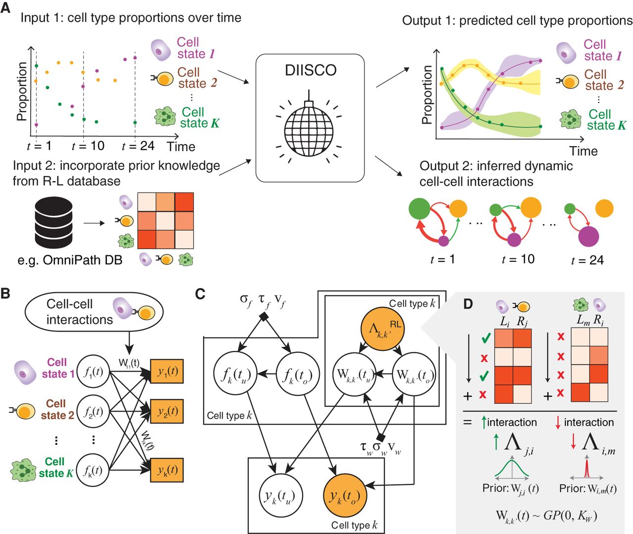
Our first assumption is that cell–cell communication, especially if associated with response to external perturbation, can be reflected in compositional shifts in cell states. In other words, a positive or negative temporal correlation between two cell states may be indicative of an activating or inhibitory interaction between them, respectively. Our second assumption is that differential gene expression of R–L complexes by these correlated cell types reinforces the likelihood of direct cell–cell communication. To improve predictive power in time intervals with low cell numbers, we integrate time-series data and encode temporal dependencies between interaction networks at different time points. By simultaneously fitting the model to all detected cell states and all time points, the algorithm effectively identifies the best sender cell state communicating with each receiver cell state, and leverages data observed in other time points, particularly the closest ones to improve prediction at a given time point. The output of DIISCO is twofold. It includes predicted cell type dynamics which is helpful for assessing model fit, for example, when tuning hyperparameters. Additionally, DIISCO outputs a time-series interaction matrix that reveals which cell–cell interactions are evolving with time (Fig. 1A).

At its core, DIISCO utilizes a generative model. To capture the temporal dynamics of cell types, that is, changes in their frequency over time, while addressing the challenge of varying time intervals, we deploy Gaussian process (GP) regression models (Wilson et al. 2012; Methods). GPs provide sufficient flexibility with nonparametric function learning, and therefore do not require any knowledge of form or rate of changes of cell types, thus expanding their applicability. They have been proven successful in integrating time-series single-cell data sets (Lönnberg et al. 2017), and in identifying key cell states with distinct temporal dynamics shaping response to immunotherapy in human leukemia (Bachireddy et al. 2021). By utilizing GPs, which encode temporal dependencies between all pairs of time points, we expand the utility of the model not only to controlled experimental settings but also to scenarios with variable timing (e.g., patient data).

To encode dynamic interactions between cell types (Fig. 1B), we draw inspiration from Gaussian process regression networks (GPRNs) that have been previously applied to gene expression dynamics as well as data sets in finance, physics, geostatistics, and air pollution (Wilson et al. 2012; Li et al. 2020). GPRNs are Bayesian multioutput regression networks that leverage the flexibility and interpretability of GPs as well as the structural properties of neural networks. The ability to capture highly nonlinear and time-dependent correlations between outputs makes GPRNs ideal for learning complex cell–cell interactions and their variability over time (Fig. 1C; Methods). Although previous methods have applied GPs to learning cell type dynamics in time-series single-cell data (Bachireddy et al. 2021), our method is the first to utilize a GPRN framework for learning interactions between cell types, rather than learning the dynamics of each cell type independently.

Finally, DIISCO utilizes an optional prior based on the expression of receptor–ligands (R–Ls) and learns interactions from both R–L gene pairs and temporal dynamics of cell types, while reliance on R–Ls can be adjusted with the prior strength (Fig. 1D; Methods). Utilizing the R–Ls is beneficial for constraining the solution space of interactions and improving model identifiability and robustness.

DIISCO recovers time-resolved interactions in synthetic data

We first evaluated the performance of DIISCO on synthetic data by constructing a data set with known dynamics and interactions (Methods). We observe an accurate modeling of temporal dynamics for five simulated cell states, even with volatile dynamics and nonuniform sampling of time points (Fig. 2A,C).

Figure 2.

Simulated data and results. (A) Simulated data for 5 cell types generated using the process described in Methods with noise parameter set to 0.1 and 40 sampled time points. Nonuniform sampling of time points increases complexity. Dots represent data points for each of the 5 cell types. The orange line is the average learned DIISCO dynamics after fitting the data over 1000 samplings. The shaded region shows 95% confidence intervals. No normalization was used. (B) Interactions inferred by DIISCO between the cell types are shown in (A). Ground truth W interactions are shown in dotted lines whereas DIISCO predictions are solid lines. Only dynamic interactions with W(t) > 0.1 in at least one time point t for either true W or learned W are shown. (C) Same as in A, except noise parameter set to 0.5. (D) Same as in B, except learned interactions for the noisier data set shown in (C). (E) Method robustness to number of time points: R² calculated between inferred and ground truth W(t). Mean and SD across five iterations are shown. (F) Runtime for varying numbers of clusters and time points. (G) Table demonstrating DIISCO performance compared to linear model (LM) and rolling linear model (RLM) as described in Methods for 40 time points. Metrics for different numbers of time points from 10 to 90 can be found in Supplemental Tables S1 and S2. Each model was tested over 10 iterations and mean and SD are shown for each metric across all iterations. Model acronyms denote the following: (LM) linear model with prior, (LM_nop) linear model, (RLM) rolling linear model with prior, (RLM_nop) rolling linear model. Model details can be found in Methods. Comparison metrics used are as follows: $R^2\mathrm{\_}Y$, $R^2\mathrm{\_}W$: R² value comparing predictions to ground truth for dynamics (Y) or interactions (W). Higher is better. $\mathrm{RMSE\_}Y$, $\mathrm{RMSE\_}W$: Root mean squared error for dynamics (Y) or interactions (W). Lower is better. (AUC) area under ROC curve. Higher is better. (AUPRC) area under precision–recall curve. Higher is better. F1: Max F1 score. Higher is better. AUC, AUPRC, and F1 scores were calculated by comparing predicted interactions to ground truth interactions.

Open in new tabDownload PowerPointLink to figure

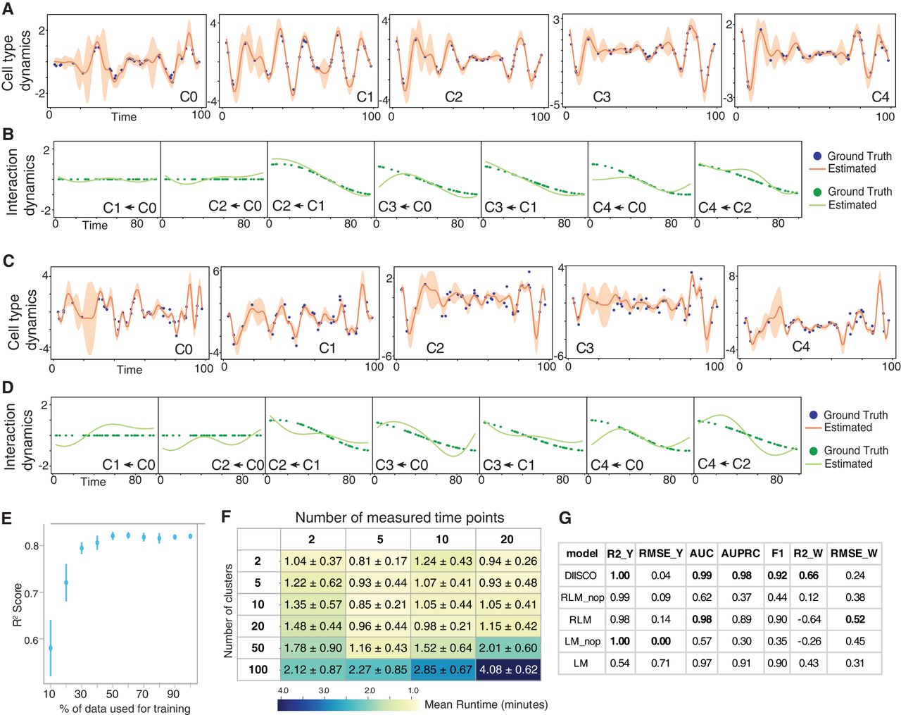
Through these simulations, we noted DIISCO's ability to uncover a wide range of interactions, including constant interactions, monotonically increasing or decreasing interactions, as well as transient interactions (Fig. 2B,D). Distinguishing various forms of interactions is important in biological data, especially in studying the impacts of perturbations and disease progression, and in resolving the timing of critical cross talk. In the case of disease progression, interactions between cell types may steadily increase or decrease over time (such as in C4 ← C0 and C2 ← C1), for example, as malignant cells become more prominent or immune cells exhibit clonal expansion. Recapitulating these complex interactions by DIISCO demonstrates its potential to derive insights into dynamic cell communication.

Because sparse sampling of time points can typically occur in real-world scenarios, particularly with clinical samples, we evaluated the robustness of our method to the number of time points. We repeated the described experiment with removing a random subset of time points, ranging from 0% to 90%, and observed sustained performance even with 70% of time points removed (Fig. 2E). We also tested the scalability of DIISCO by increasing the number of clusters and time points (Fig. 2F), as well as analyzing the algorithmic complexity of DIISCO (Methods). Our empirical assessment of scalability confirmed exponential scaling with the number of cell types and time points; however, we still observe run times <5 min for 100 simulated clusters and 20 time points using a Google Cloud machine instance with 117 GB of RAM and 30 cores (Fig. 2D). This scalability suggests DIISCO would be able to provide insight into large-scale temporal cell atlases, should they become available.

To further benchmark DIISCO's ability to infer temporal dynamics and interactions, we compared DIISCO's performance to both a linear model and a rolling linear model (Methods). We also tested the importance of the prior, by comparing to models with and without a prior incorporated. By simulating various scenarios with differing time points and noise (Methods), we confirmed that DIISCO accurately reconstructs temporal changes, and demonstrates superior performance in predicting interactions compared to baseline models without the prior (Fig. 2G; Supplemental Tables S1, S2). The performance in predicting interactions between cell types at measured time points becomes comparable to the rolling linear model if the DIISCO prior is incorporated, underscoring the impact of promoting sparsity in the interaction network. However, the baseline models are yet incapable of interpolating interactions between measured time points, limiting the evaluation of interaction dynamics over time. They are also unable to identify R–Ls or gene programs correlated with time-resolved cell type interactions. Overall, DIISCO performs both tasks of inferring smooth time-dependent interactions without assumptions about functional form and incorporating prior knowledge in an integrated Bayesian framework, while quantifying uncertainty and enabling downstream analysis of underlying mechanisms. This is an essential feature for biological applications and hypothesis generation for future investigations.

DIISCO characterizes dynamic interactions between CAR T and lymphoma cells

To demonstrate an application of DIISCO to biological data, we generated single-cell data from a controlled in vitro experimental setting. Specifically, we cocultured green fluorescent protein (GFP)-transduced anti-CD19 (CAR T cells together with MEC1 cells (Stacchini et al. 1999)—a B cell (chronic lymphocytic leukemia [CLL]) leukemia cell line expressing CD19—as the CAR T cell target (Fig. 3A; Supplemental Fig. S1A–C; Methods). We confirmed dose response activation (cytotoxicity) of T cells by quantifying the percentage of remaining MEC1 cells. This showed a reduction in MEC1 cell survival starting from 50% to 60% at an effector-to-target ratio of 0.125 to survival of <5% at an effector-to-target ratio of 4 (Supplemental Fig. S1D). We profiled four biological replicates with scRNA-seq at 10 time points spanning 24 h, thereby obtaining high-quality data for 49,283 total cells (Supplemental Table S3). The data show compositional shifts with time, motivating the use of this data set as a test case for investigating temporal interactions with DIISCO (Fig. 3B).

Figure 3.

CAR T experimental setup and data preprocessing. (A) Overview of the data collection process and analysis of coculture experiments outlined in Supplemental Table S1. (B–D) 2D UMAP projection of 9082 single-cell transcriptomes from Experiment C colored by time point (B), cluster and cell type assignment (C), and average expression of different gene set markers (D) used to define metaclusters. (E) Heatmap of average cluster expression of individual genes used in gene set analysis, Z-scored across all clusters. (F) Prior constructed for DIISCO input, generated as explained in Methods.

Open in new tabDownload PowerPointLink to figure

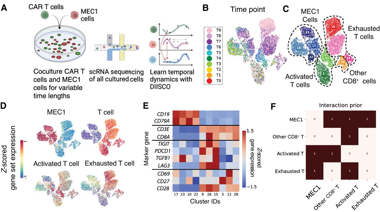
We preprocessed this data by defining major cell types from the combination of all replicate experiments to increase statistical power. Through clustering and examining the expression of curated gene sets, we identified four major cell types (metaclusters): cancer cells, exhausted CD8⁺ T cells, activated CD8⁺ T cells, and other CD8⁺ T cells showing neither activated nor exhausted markers. MEC1 cancer cells were annotated based on the expression of CD19 and CD79A. T cells were annotated based on the expression of CD3E, CD3D, and CD8A. Activated T cells were defined by expression of CD69, CD27, and CD28, whereas exhausted cells were defined by expression of TIGIT, PDCD1, TGFB1, and LAG3 (Fig. 3C–E). Clusters that were positive for both T cell and MEC1 gene markers were removed as doublets. We acknowledge that doublets could also contain interacting cells. However, because we only obtain one measurement of receptor or ligand gene, our current method (as well as existing methods) cannot resolve them. Future extensions deploying mixture models could help deconvolve doublets.

After cell type annotation, proportions were calculated at each time point, and DIISCO was trained on each experiment separately (Supplemental Fig. S2A,C). To construct the prior for interactions, we obtained a set of 8234 literature-curated R–L pairs from OmniPath, a database of cell signaling prior knowledge (Türei et al. 2016) and summarized the number of R–Ls with differential expression between each pair of cell types (Fig. 3F; Methods).

Applied to the CAR T and MEC1 data, DIISCO learned the proportions of cell types, highlighting the expected decrease in cancer cells over time and the increase in exhausted T cells (Fig. 4A; Supplemental Fig. S2A,C). We also inferred interactions between cell types and specifically observed strong negative interactions predicted between cancer cells and exhausted CAR T cells, as well as between activated and exhausted T cells (Fig. 4B,C; Supplemental Fig. S2B,D). Investigating the dynamics of interactions W(t) over time, as expected, we predicted an increase in the strength of the interaction (|W|) with coculture time (Fig. 4C) between exhausted T cells and MEC1 cells, as well as in exhausted T cells interacting with activated T cells, which was directionally specific. The former recapitulated the targeting of cancer cells by T cells and the latter may be due to phenotypic shifts from activated T cells becoming more exhausted or terminally differentiated over time (Bachireddy et al. 2021). When comparing DIISCO results across experiments, we note that the predicted interactions (W) between cell types averaged over time remain consistent for the strongest positive and negative interactions (Supplemental Fig. S2E). Furthermore, the main interaction links between exhausted T cell–MEC1 and exhausted–activated T cells exhibit the same time-varying dynamics across experiments, demonstrating DIISCO's robustness and reproducibility across biological replicates (Supplemental Fig. S2F,G). One benefit of DIISCO is its ability to provide uncertainty estimates in interaction predictions, and we note that the uncertainty, as defined by one standard deviation, increases after 12 h, due to increased sparsity in collected time points (Supplemental Fig. S3).

Figure 4.

DIISCO performance on CAR T Experiment C. (A) Temporal dynamics of cell types. Data points represent the measured proportion of cell types over time, and DIISCO output is shown as inferred mean (solid line) and one standard deviation (shaded area) of y for each cell type. Additional experiments are shown in Supplemental Figure S2. (B,C) Inferred W interaction matrix at two example time points (B) and over the entire coculture time window (C). Network node size reflects cell type proportion at that time point; arrows and their width designate the direction and strength of inferred interactions, respectively. (D) Average interaction strength between clusters as a function of varying prior thresholds. The binarization threshold indicates the minimum number of R–L interactions between two cluster pairs needed to denote a 1 in the prior matrix. (E) Rank of average interaction strengths as a function of varying prior thresholds. (F) Average interaction score with downsampling total cell number. (G,H) W interaction over time between exhausted T cell and MEC1 cells (G) and exhausted–activated T cells (H) for different percentages of dropped cells.

Open in new tabDownload PowerPointLink to figure

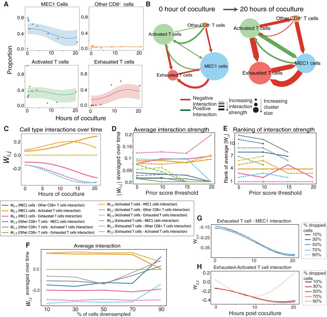
The ability to predict how interactions between exhausted T cells and MEC1 cells evolve with time is a unique feature of DIISCO, whereas other existing methods are not able to achieve such time-resolved predictions. Indeed, we observed a positive correlation between predicted interaction strength and coculture time (Fig. 4C), in line with the cytotoxicity of T cells, that is, their increased ability to kill cancer cells.

Additionally, we assessed the sensitivity of DIISCO to the interaction prior by changing the interaction score threshold that we used for quantifying the number of possible R–L complexes associated with a pair of cell states. A lower threshold would lead to a larger solution space, whereas higher thresholds emphasize clusters with the largest number of expressed R–L genes. We noted that the average interaction strength predicted by DIISCO remained stable, excluding the interactions that drop out with higher thresholds (Fig. 4D). Importantly, the ranking of most strongest predicted interactions remained stable (Fig. 4E).

To assess the sensitivity of DIISCO to the number of cells, we downsampled the cells in this data set and observed robust ranking of interactions even when cells are downsampled to 30% of the original numbers, with only minor changes when downsampling 40%–50% of cells (Fig. 4F–H; Supplemental Fig. S4A). To additionally test sensitivity to user input, we also downsampled the time points in this data set (Supplemental Fig. S4B). DIISCO recovers similar dynamics even with 50% of time points dropped. Tracking the average interaction strengths over time, we see robust estimations even with 30% of time points dropped (Supplemental Fig. S4C). This is also evident in the time-varying dynamics of these interactions (Supplemental Fig. S4D,E). We additionally sought to test sensitivity to clustering techniques, as users may utilize different preprocessing pipelines. We first tested DIISCO's performance on the individual PhenoGraph clusters without merging them into metaclusters. The results show MEC1 cells (clusters 10, 17, 22, and 23) have a decrease in proportion after 10 h post-coculture (Supplemental Fig. S5A). Activated T cells (clusters 3 and 12) show higher proportions early in the experiment and then decrease over time. This complements the dynamics of exhausted T cells (clusters 9, 15, and 26) which are increasing over time.

Examining the average W interactions over time, C10 → C26 and C10 → C9 are the strongest negative interactions (Supplemental Fig. S5B,C). These are both MEC–exhausted T cell links consistent with our previous results at the level of metaclusters. The strongest positive interactions belong to C23 → C9, C9 → C23, and C26 → C9. These are MEC–exhausted T cell and exhausted T cell–exhausted T cell interactions. These results demonstrate DIISCO's robustness to various clustering methods and varying data quality. One benefit to combining clusters into metaclusters that define individual cell types is the ability to remove any self-interactions. With multiple clusters representing exhausted T cells, we see interactions between different exhausted T cell clusters arise. Although there are cases where this may be important to study, DIISCO has been built to study intercellular interactions between different cell types, instead of within them. We also demonstrate DIISCO's robustness to the clustering method by reprocessing the data following SCANPY's pipeline, including Leiden clustering to define cell types (Methods). We see similar results in both dynamics and predicted interactions (Supplemental Fig. S5D–F).

DIISCO outperforms existing methods in identifying cell communication mediated by signaling molecules

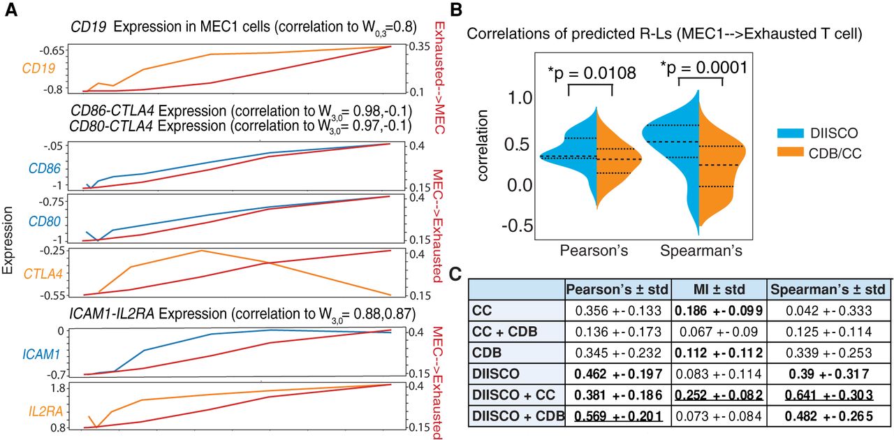
To investigate mechanisms underlying the interaction between MEC1 cells and exhausted T cells in our in vitro experiment, we calculated the correlations between different R–L gene pairs and the learned dynamic interaction (Fig. 5A). For calibration, we first confirmed that CD19, the target of the engineered CAR, is highly correlated with the interaction from exhausted T cells to MEC1 cells, as expected (Fig. 5A). Examining the MEC1 → exhausted interaction, CD86–CTLA4 and CD80–CTLA4 were the top R–L pairs ranked by ligand correlation (Fig. 5A). CTLA4 is an established marker of T cell exhaustion, and CD80 and CD86 are costimulatory molecules that are expressed in malignant lymphocytes (including B cells) in several hematologic diseases (Delabie et al. 1993; Dorfman et al. 1997; Vyth-Dreese et al. 1998). Ranked by the highest average correlation, ICAM1–IL2RA was the top predicted R–L pair. ICAM1 is a known regulator of inflammatory response and is elevated in CLL patients with more severe disease progression (Molica et al. 1995; Musolino et al. 1996; Bui et al. 2020).

Figure 5.

Comparing predicted R–L pairs with existing methods. (A) R–L pairs are highly correlated with DIISCO-predicted W_{exhausted↔MEC} interaction. Expression of ligands is shown in blue, receptors in orange (left axis), and interaction strength in red (right axis). (B) Comparison of DIISCO-predicted R–L pairs with those predicted using CellChat (CC) or CellPhoneDB (CDB). Correlations between paired R–Ls are shown for the W_{MEC→exhausted T cell} link. P-values calculated with the Mann–Whitney U test. (C) Evaluating temporal correlation of predicted R–Ls using each method: DIISCO, CDB, and CC. A + B refer to R–L pairs predicted by methods A and B. Table shows three different metrics calculated for all R–L pairs: Pearson's correlation, mutual information (MI), and Spearman's correlation. Mean values ± SD are quantified, with the top three highest scores in bold and the highest score underlined.

Open in new tabDownload PowerPointLink to figure

Finally, we benchmarked the predicted DIISCO R–L interactions against other methods including CellChat (Jin et al. 2021) and CellPhoneDB (Efremova et al. 2020). We applied CellPhoneDB and CellChat to log-normalized expression data from all time points. We excluded any interactions within the same cluster (i.e., MEC1 → MEC1). R–L pairs were filtered based on P-value (P < 0.05), and we identified 260 significant pairs using CellPhoneDB and 180 significant interactions using CellChat.

To compare these results to DIISCO-predicted interactions, we calculated the correlation between the predicted receptor and ligand expression over all time points. Our rationale is that if R–L protein complexes mediate cell–cell interaction, their expression levels on the corresponding sender and receiver cell types will likely change concomitantly. Otherwise, the genes are less likely to be involved in the cellular interaction and could rather be intrinsic markers of the cell states. We observed a significantly higher Pearson's correlation for R–Ls in DIISCO-predicted interactions than those predicted by other methods (Fig. 5B). Because changes in the expression of receptor genes on the receiver cell type may not be linearly associated with the corresponding ligand expression on the sender, we also calculated Spearman's correlation, again demonstrating a significant improvement with DIISCO (Fig. 5B). Although all three methods identified the CD80/CD86–CTLA4 interactions, only DIISCO predicted the ICAM1–IL2RA interaction, which is the one with the most time-varying expression. Note that temporal changes in the expression of R–L genes are not used in the DIISCO prior. Our results thus confirm the ability of DIISCO to identify a monotonic increase in the expression of R–L pairs underlying cell–cell interactions.

Further examining the overlap between methods, we noted that the predicted interactions shared between DIISCO and CellChat are the most correlated by both Spearman's correlation and mutual information as another metric, whereas the interactions predicted by both DIISCO and CellPhoneDB are most correlated using the Pearson's correlation test (Fig. 5C). Combined, these results confirm DIISCO's ability to identify cell–cell communication that can be supported by coexpressed R–L gene pairs, from time-series single-cell data.

As DIISCO learns interactions from the integration of time-series data, we further compared DIISCO to CellPhoneDB applied to different time points. Due to low numbers of cells in metaclusters in individual time points, we were unable to apply CellPhoneDB to each time point separately. Instead, we combined the first 5 and last 4 time points into “early” and “late” time intervals to obtain pseudo-dynamic interactions. Identifying R–L pairs that were only predicted in the “late” bucket suggests that these interactions are growing in strength over time. Predicted R–L interactions between MEC1–exhausted cells found with both DIISCO and the “late” bucket in CellPhoneDB include TNF-ICOS, FAM3C-PDCD1, and FAM3C-LAMP1. ICOS is known to be expressed on activated T cells, and it has been investigated as a costimulatory domain for CAR T cell therapy (He et al. 2022). High expression of TNF in CLL cells has been associated with poor prognosis, and TNF has been suggested as a potential target for CLL immunotherapies (Dürr et al. 2018). Even with the bucketing approach CellPhoneDB did not predict CD80/CD86–CTLA4 interactions, which have strong literature support for their importance in CLL (Delabie et al. 1993; Dorfman et al. 1997; Vyth-Dreese et al. 1998). CellPhoneDB also did not identify the ICAM1–IL2RA interaction. This suggests that incorporating temporal dynamics is crucial for identifying R–L interactions most relevant to the biological system.

Notations

We assume that we have K cell types with their frequencies measured at time points t₁, …, t_N. We define y(t_i) as a K-dimensional vector of observations at time t_i where the kth dimension corresponds to the frequency of the kth cell type. Additionally, we assume we have a set of M unobserved time points t_N+1, …, t_N+M, placed anywhere on the time axis, for which we would like to infer (interpolate) the cell type values y(t_N+1), …, y(t_N+M). We denote the set of all time points as $\mathcal{T}=\{t_1,\dots ,t_{N+M}\}$ and call ${\mathcal{T}}_u$ the set of unobserved time points ${\mathcal{T}}_u=\{t_{N+1},\dots ,t_{N+M}\}$ and ${\mathcal{T}}_o$ the set of observed time points ${\mathcal{T}}_o=\{t_1,\dots ,t_N\}$. We use the convention of ·_u and ·_o to denote unobserved and observed variables, respectively. In the remainder, for ease of exposition, we will refer to y(t_i) as proportions with the understanding that either proportions or cell counts could be used, although the results should be interpreted in a different manner depending on the value used.

In addition to these features, we have a binary matrix Λ of size K × K where ${\mathit{\Lambda }}_{k,k^{\mathrm{\prime }}}=1$ indicates that the kth cell type might interact with the $k^{\mathrm{\prime }}$th cell type and ${\mathit{\Lambda }}_{k,k^{\mathrm{\prime }}}=0$ indicates that they do not. We allow for nonsymmetric matrices to allow for directionality in interactions. In practice, we obtain this matrix from measurements of expression of known R–L complexes.

Model specification

DIISCO is a generative model that assumes cell type frequencies, denoted as $\hat{y}\left(t_i\right)$, are derived from the following process (Fig. 1B):

Figure 1C depicts this process graphically and Algorithm 1 details the generative process. The arrows ${\mathcal{W}}_o\to {\mathcal{W}}_u$ and ${\mathcal{F}}_o\to {\mathcal{F}}_u$ represent tractable distributions that can be computed analytically and can be sampled due to the properties of GPs. Thus, the model only requires tractable operations that lead to the joint distribution described. DIISCO currently ignores the original space that the data lies in and makes the simplifying assumption that y(t) can be treated as a vector in ℝ^k rather than on the simplex or the space of positive integers. Although these assumptions aid greatly in the interpretability of the latent variables, further improvements using distributions that truly match the real support of the data would lead to better uncertainty estimates and predictions.

Model interpretation

The latent variable W_i,j(t) represents the direction and effect of intercellular interaction (signaling communication) from cell type j to cell type i at time t. In particular, W_i,j(t) > 0 represents an activating effect, W_i,j(t) < 0 denotes inhibitory impact, and |W_i,j(t)| reflects the strength of the interaction. f(t)_i is a latent variable that represents the normalized proportion of cell type i at time t (Fig. 1B). DIISCO focuses on identifying interactions between different cell states. Thus, in constructing the prior for W, we penalize self-interactions W_i,i, such that W_i,j can be interpreted as the impact of other cell types j ≠ i on the dynamics of cell type i. We justify why this interpretation is reasonable, given our choice of priors below.

Prior distribution over F

Intuitively, we aim for the latent features to align closely with standardized cell type proportions so that W(t), with suitable restrictions on the diagonal, learns to capture the interactions between cell types by predicting the standardized proportion of one cell type given the standardized proportions of the rest. We achieve this by first defining for every feature an auxiliary zero-mean GP on which we perform inference. Formally, for every k ∈ {1, …, K}, we define an auxiliary GP with covariance function K^f given by

Prior distribution over W

To further limit the solution space, and improve model robustness and interpretability, we set two constraints on the sampling process of W. First, we set off-diagonal elements to zero if the cluster pairs do not express any complementary R–L pairs and second, we zero out the diagonals when a row has at least one other nonzero entry. In the case when we are dealing with proportions and not raw counts, this also ensures that we avoid a trivial solution due to the $\sum _k{y}_k\left(t\right)=1$. Formally, we achieve this by sampling W(t) so that for $k,k^{\mathrm{\prime }}\in \{1,\dots ,K\}$.

We then quantify the number of these interactions expressed by cluster pairs. The number of R–L pairs does not necessarily determine the strength of interaction, and a single complementary R–L pair could be biologically important. To account for this, we set a binarization threshold. The binarization threshold can be set by users and may be datatype-specific. A very high threshold leads to a prior that is too sparse and may lead to losing potentially relevant interactions, whereas a very low threshold may lead to spurious interactions. The threshold is user-specified and determines the sparsity of the prior during the binarization step.

To demonstrate the robustness of predicted interactions to the threshold, we performed additional sensitivity analysis by dropping 30%–70% of the R–L pairs in the OmniPath R–L database. When we drop different percentages of R–L pairs, we obtain a similar distribution of interaction scores (Supplemental Fig. S6A–C). By specifying a threshold guided by the knee point of these distributions, we achieve the same prior using 30% or 70% of the data. By changing the threshold to account for downsampled or incomplete interactions, we can retain flexibility in the model and utilize a consistent prior. Unfortunately, similar to current interaction methods like CellPhoneDB or CellChat, if there is a bias in the database where certain cell types are underrepresented, we are unable to capture that in the predicted results. Future databases expanding these interactions can improve results obtained with DIISCO.

By binarizing the R–L interaction matrix, we allow for more model flexibility while also limiting the solution space to exclude clusters with no complementary R–L expression. This final binary matrix is defined as Λ, and as shown in Equation 4, the value of ${\mathit{\Lambda }}_{k,k^{\mathrm{\prime }}}$ determines whether the model allows for a possible interaction between cell types k and $k^{\mathrm{\prime }}$. In practice, we build the prior using OmniPathDB, a database used by more traditional interaction methods like CellPhoneDB (Türei et al. 2016). However, it is important to note that R–L databases lack context-dependent information and are often incomplete with many interactions having not been characterized yet in literature.

Inference

Due to the complex nature of the model, it is not possible to perform inference analytically. Instead, we deploy a two-step approximate inference method combining both analytic and approximate techniques.

Specifically, we: (1) perform approximate inference to obtain samples from an estimate of the posterior distribution $p({\mathcal{W}}_o,{\mathcal{F}}_o\mid {\mathcal{Y}}_o)$; and (2) perform ancestral sampling and standard GP conditioning to obtain an approximation to the posterior distribution $p({\mathcal{W}}_u,{\mathcal{F}}_u,{\mathcal{Y}}_u\mid {\mathcal{Y}}_o,{\mathcal{W}}_o,{\mathcal{F}}_o)$. Supplemental Information Section B provides a justification for this approach. Below we describe in detail how we perform each of these steps.

Approximate inference

To approximate $p({\mathcal{W}}_o,{\mathcal{F}}_o\mid {\mathcal{Y}}_o)$, we use variational inference implemented using Pyro (Bingham et al. 2019), a probabilistic programming language written in Python. Within this framework, we define a parameterized distribution $q_{\varphi }({\mathcal{W}}_o,{\mathcal{F}}_o)$ and then optimize the parameters ϕ to maximize an estimate of the evidence lower bound (ELBO) (Blei et al. 2017) via a gradient descent algorithm. In the situation where the hyperparameters are fixed, this is equivalent to minimizing the KL divergence $\mathrm{KL}\left(q_{\varphi }({\mathcal{W}}_o,{\mathcal{F}}_o)\left|\right|p({\mathcal{W}}_o,{\mathcal{F}}_o|{\mathcal{Y}}_o)\right)$.

In this case, the ELBO is given by

In other words, we assume that the latent features and the interaction matrix are independent of each other, but they are dependent across time points, and this dependency is captured by the mean and covariance of the Gaussian distribution. In practice, we parameterize the Cholesky decomposition of the covariance matrix rather than the covariance matrix itself and use Adam (Kingma and Ba 2017) to optimize the parameters ϕ. Due to the amount of computation required for using this variational family, we also provide in the package the option to use a mean-field guide where each variable is fully independent from the others and is parameterized by a one-dimensional normal distribution, where $q_{\varphi }({\mathcal{W}}_o,{\mathcal{F}}_o)=\prod _{z\in {\mathcal{W}}_o\cup {\mathcal{F}}_o}q\left(z\right|{\mu }_z,{\sigma }_z)$. We refer to the family with the time-wise dependency structure as the partially factorized variational family, and the one with a full diagonal covariance as the fully factorized variational family.

To perform optimization, we used an expectation with the form $\mathbb{E}{q}_{\varphi \left(Z\right)}\left[h_{\varphi }\right(Z\left)\right]$ where $Z=({\mathcal{W}}_o,{\mathcal{F}}_0)$ and h represents the function inside of the expectation in Equation 5. This is problematic for taking the gradient with respect to ϕ because it appears both in the distribution with respect to which we are taking the expectation and in h. However, using the fact that if L = Cholesky(Σ), $\epsilon \sim \mathcal{N}(0,I_d)$ and $z=\mu +\mathrm{\Sigma }\epsilon$ then z must be distributed as $\mathcal{N}(\mu ,\mathrm{\Sigma })$, it is easy to see that one can rewrite the expectation as $E_{\mathcal{D}\left(\epsilon \right)}\left[h\right(z(\epsilon ,\varphi )\left)\right]$ where D is a multivariate normal distribution with identity covariance and $z(\epsilon ,\varphi )$ maps this random variable to the equivalent Z values using the above approach. We use this reparameterization trick (Kingma and Welling 2022) to construct and estimate the gradient of the ELBO. Supplemental Information Section C outlines the inference algorithm and provides details of ancestral sampling.

Algorithmic complexity and scalability

An important consideration for GP-based models is their scalability and time complexity. For DIISCO, using either variational family, the computational complexity of approximate inference is of the order $O\left(\right|{\mathcal{T}}_o{|}^3{K}^2)$ per gradient step and the exact conditioning step leads to a computational complexity of $O\left(K^2\right(|{\mathcal{T}}_o{|}^3+|{\mathcal{T}}_o{|}^2\left|{\mathcal{T}}_u\right|\left)\right)$ for either sampling or computing the means. Supplemental Information Section F details which exact operations lead to the above bounds.

Nevertheless, for most of the data sets that could appear in practice the algorithmic complexity is not an issue, especially when using the fully factorized normal guide. To demonstrate this, we ran DIISCO on various simulated data sets with different sizes of ${\mathcal{T}}_o$ and K to benchmark the performance. Specifically, we constructed the data sets by sampling the K GPs with half of the processes being independently sampled and the other half being a linear combination of the independent ones. The values for the linear combination were also sampled from a GP with 10 times the length scale of the independent ones, which was set to 1. To simulate sparsity for every nonindependent process, we selected at random a number between 0 and floor(K/2) and then proceeded to zero out that many values in the linear combination. The observed time points were sampled uniformly between 0 and 10. We then ran DIISCO for up to 50,000 iterations with early stopping if there were no improvements for over a 1000 iterations. We conducted these experiments on a Google Cloud machine instance with 117 GB of RAM and 30 cores. Figure 2F shows that the run-time remains under 5 min even when fitting to up to 100 clusters and 20 time points, which are reasonable dimensions for comprehensive time-series single-cell data sets.

Benchmarking with simulated data

To understand the behavior of DIISCO under different scenarios, we conducted a benchmarking experiment using simulated data. We specifically aimed to evaluate the ability to predict interactions with nonzero strength. Details of this process are provided below.

CAR T data collection

CD19 CAR T cells were generated by transducing healthy donor T cells with third generation lentiviral vectors encoding a bicistronic construct containing either FMC63 CD19 scFv-CD28-CD3ZETA (currently known as CD247) and GFP or FMC63 CD19 scFv-41BB-CD3ZETA (Supplemental Fig. S1A; Nicholson et al. 1997). Peripheral blood mononuclear cells were resuspended at 2 × 10⁶/mL and seeded at 1 mL per 24-well plate and activated with CD3/CD28 Beads. The next day, fresh media was added with IL2 to a final concentration of 100 IU/mL. Six hours later cells were harvested, counted, and resuspended at 0.6 × 10⁶/mL, and 0.5 mL was seeded into a 24-well plate precoated with RetroNectin (Supplemental Fig. S1C); 1.5 mL of lentiviral supernatant was added to each well with fresh IL2 to a final concentration of 100 IU/mL and spun for 40 min at 1000G. Two days later cells were harvested, resuspended at 0.5 × 10⁶/mL with 50 IU/mL of IL2 and left to expand and split every 48 h. Transduction efficiency was assessed by determining the percentage of GFP⁺ T cells.

Cocultures of CD19 CAR T cells and MEC1 cell line (ATCC), a CLL cell line that constitutively expresses CD19, were established at various effector-to-target ratios and at different time points (Supplemental Table S3). Cocultures were harvested together and stained with hashing antibodies (Biolegend), normalized, and prepared for scRNA-seq on the 10x Genomics Chromium platform. Experimental details for each of the four experiments are found in Supplemental Table S3.

CAR T data preprocessing and analysis

Each coculture experiment was hashed by time point according to Supplemental Table S3. Demultiplexing was done in R as detailed below: All cells with <200 detected UMIs were removed as empty droplets. For each cell, hashtag oligos (HTOs) were ranked according to detected counts, and the standard deviation and mean for HTOs ranked 2–4 were calculated. Cells were removed if the difference between HTO2 and HTO3 were within 1 SD and if HTO2 was within 15% of the mean of HTO2–4. Finally, the top 2 HTOs for each cell were used as cell identifiers and matched based on Supplemental Table S3.

All count data across all four experiments was aggregated and log-normalized as (log(0.1 + counts)). Data were visualized by UMAP, based on principal component analysis (PCA) with eight components. Clustering was performed on 15 PCA components, using PhenoGraph (Levine et al. 2015) and a k-nearest neighbor (kNN) with n = 15. Thirty clusters were found, and then separated into four different metaclusters. MEC1 cells (clusters 1, 7 8, 10, 17, 22, 23, and 24) were defined based on differential expression of IKGC, CD79A, MS4A1, and CD19. T cells were defined based on differential expression of CD3D and CD3E. Exhausted T cells (clusters 0, 6, 9, 11, 15, 21, and 26) were defined based on TIGIT, CTLA4, PDCD1, IL10, TGFB1, LAG3, and activated cells defined based on the expression of CD69, CD27, and CD28. Any CD8⁺ cells that did not express activation or exhaustion signatures were grouped into a separate fourth category (clusters 19 and 28). The following clusters were removed as doublets: 2, 11, 14, 16, 20. All other clusters were removed due to low library size.

To construct Λ, we first obtained a set of 8234 literature-curated R–L pairs from OmniPath, a database of cell signaling prior knowledge (Türei et al. 2016). For each cell type pair $k,k^{\mathrm{\prime }}$ in the experiment, we quantified interactions as the number of differentially expressed ligand genes in cell type k with their corresponding differentially expressed receptor genes in cell type $k^{\mathrm{\prime }}$ at each time point. These interaction count values were averaged across all time points in the experiment and then thresholded to obtain the binary interaction prior matrix Λ, where ${\mathit{\Lambda }}_{k,k^{\mathrm{\prime }}}$ signifies whether cell types k and $k^{\mathrm{\prime }}$ can interact a priori. The threshold was chosen with a data-driven approach according to the knee point of sorted values.

CAR T data preprocessing—Leiden comparison

Count data for all CAR T replicates was aggregated and filtered according to the SCANPY scRNA preprocessing tutorial (https://scanpy.readthedocs.io/en/stable/tutorials/basics/clustering.html). Cells expressing <100 genes were removed, and any genes expressed in <3 cells were removed. Scrublet was then used, via scanpy.external.pp.scrublet() function to remove doublets. Data were log normalized. The kNN neighbor graph was built on 20 PCA components and 10 neighbors, and Leiden clustering was then used to define clusters with the resolution set to 0.5. Clusters were then sorted into cell types based on gene expression. T cells were assigned based on expression of CD3E, and CD3D. Clusters 5 and 6 were designated as exhausted T cells based on the expression of TIGIT, CTLA4, PDCD1, IL10, TGFB1, and LAG3. Clusters 7, 9, and 17 were assigned as activated T cells based on expression of CD69, CD27, and CD28. Clusters 0, 3, 4, 11, 14, and 15 were designated as MEC1 cells based on the expression of IGKC, CD79A, MS4A1, and CD19. Clusters 1, 2, 13, and 16 were designated as Other CD8⁺ T cells, and clusters 8 and 10 were labeled as additional doublets and removed due to contradictory expression of both T cell and MEC1 markers. Proportions were calculated by normalizing to total numbers of cells in clusters.

DIISCO design parameters

R–L comparison

CellPhoneDB version 2.0.0 was applied to generate interactions in Experiment C. To filter predicted interactions, we only reported R–L pairs that had nonzero counts in the respective sender and receiver clusters and P < 0.05. For running CellChat in RStudio, we used the default human CellChat database (Jin et al. 2021; R Core Team 2022). For both methods, all time points were aggregated to increase statistical power. To compare the results between all three methods, we focused on the MEC → exhausted interaction. Spearman's and Pearson's correlations were calculated with the SciPy package, and mutual information was calculated using sklearn package for the union of all R–L pairs predicted by any of the three methods.

We further ran CellPhoneDB on “early” and “late” time points grouped together. “Early” was defined as the first 5 time points and “late” was defined as the last 4 time points. We then ran CellPhoneDB and processed the predicted interactions as mentioned above. To compare to DIISCO, we limited predicted interactions to ones that were in either the “early” or “late” set, not both. We then compared the predicted R–L pairs from DIISCO and from these two bucketed groups, identifying R–L pairs shared between both methods and ones unique to either method.

References

- ↵Azizi E, Carr AJ, Plitas G, Cornish AE, Konopacki C, Prabhakaran S, Nainys J, Wu K, Kiseliovas V, Setty M, 2018. Single-cell map of diverse immune phenotypes in the breast tumor microenvironment. Cell 174: 1293–1308.e36. 10.1016/j.cell.2018.05.060
- ↵Bachireddy P, Azizi E, Burdziak C, Nguyen VN, Ennis CS, Maurer K, Park CY, Choo ZN, Li S, Gohil SH, 2021. Mapping the evolution of T cell states during response and resistance to adoptive cellular therapy. Cell Rep 37: 109992. 10.1016/j.celrep.2021.109992
- ↵Bingham E, Chen JP, Jankowiak M, Obermeyer F, Pradhan N, Karaletsos T, Singh R, Szerlip P, Horsfall P, Goodman ND. 2019. Pyro: deep universal probabilistic programming. J Mach Learn Res 20: 973–978.
- ↵Blei DM, Kucukelbir A, McAuliffe JD. 2017. Variational inference: a review for statisticians. J Am Stat Assoc 112: 859–877. 10.1080/01621459.2017.1285773
- ↵Browaeys R, Saelens W, Saeys Y. 2020. NicheNet: modeling intercellular communication by linking ligands to target genes. Nat Methods 17: 159–162. 10.1038/s41592-019-0667-5
- ↵Bui TM, Wiesolek HL, Sumagin R. 2020. ICAM-1: a master regulator of cellular responses in inflammation, injury resolution, and tumorigenesis. J Leucoc Biol 108: 787–799. 10.1002/JLB.2MR0220-549R
- ↵Delabie J, Ceuppens J, Vandenberghe P, de Boer M, Coorevits L, De Wolf-Peeters C. 1993. The B7/BB1 antigen is expressed by Reed-Sternberg cells of Hodgkin's disease and contributes to the stimulating capacity of Hodgkin's disease-derived cell lines. Blood 82: 2845–2852. 10.1182/blood.V82.9.2845.2845
- ↵Dorfman D, Schultze J, Shahsafaei A, Michalak S, Gribben J, Freeman G, Pinkus G, Nadler L. 1997. In vivo expression of B7-1 and B7-2 by follicular lymphoma cells can prevent induction of T-cell anergy but is insufficient to induce significant T-cell proliferation. Blood 90: 4297–4306. 10.1182/blood.V90.11.4297
- ↵Dürr C, Hanna B, Schulz A, Lucas F, Zucknick M, Benner A, Clear A, Ohl S, Öztürk S, Zenz T, 2018. Tumor necrosis factor receptor signaling is a driver of chronic lymphocytic leukemia that can be therapeutically targeted by the flavonoid wogonin. Haematologica 103: 688–697. 10.3324/haematol.2017.177808
- ↵Efremova M, Vento-Tormo M, Teichmann SA, Vento-Tormo R. 2020. CellPhoneDB: inferring cell–cell communication from combined expression of multi-subunit ligand–receptor complexes. Nat Protoc 15: 1484–1506. 10.1038/s41596-020-0292-x
- ↵He Y, Vlaming M, van Meerten T, Bremer E. 2022. The implementation of TNFRSF co-stimulatory domains in CAR T cells for optimal functional activity. Cancers (Basel) 14: 299. 10.3390/cancers14020299
- ↵Jin S, Guerrero-Juarez CF, Zhang L, Chang I, Ramos R, Kuan CH, Myung P, Plikus MV, Nie Q. 2021. Inference and analysis of cell-cell communication using CellChat. Nat Commun 12: 1088. 10.1038/s41467-021-21246-9
- ↵Kingma DP, Ba J. 2017. Adam: a method for stochastic optimization. arXiv:1412.6980v9 [cs.LG]. 10.48550/arXiv.1412.6980
- ↵Kingma DP, Welling M. 2022. Auto-encoding variational Bayes. arXiv:1312.6114 [stat.ML]. 10.48550/arXiv.1312.6114
- ↵Kumar MP, Du J, Lagoudas G, Jiao Y, Sawyer A, Drummond DC, Lauffenburger DA, Raue A. 2018. Analysis of single-cell RNA-seq identifies cell-cell communication associated with tumor characteristics. Cell Rep 25: 1458–1468.e4. 10.1016/j.celrep.2018.10.047
- ↵Levine J, Simonds E, Bendall S, Davis K, El-ad D, Tadmor M, Litvin O, Fienberg H, Jager A, Zunder E, 2015. Data-driven phenotypic dissection of AML reveals progenitor-like cells that correlate with prognosis. Cell 162: 184–197. 10.1016/j.cell.2015.05.047
- ↵Li S, Xing W, Kirby M, Zhe S. 2020. Scalable variational Gaussian process regression networks. arXiv:2003.11489 [cs.LG]. 10.48550/arXiv.2003.11489
- ↵Li J, Hubisz MJ, Earlie EM, Duran MA, Hong C, Varela AA, Lettera E, Deyell M, Tavora B, Havel JJ, 2023. Non-cell-autonomous cancer progression from chromosomal instability. Nature 620: 1080–1088. 10.1038/s41586-023-06464-z
- ↵Lönnberg T, Svensson V, James KR, Fernandez-Ruiz D, Sebina I, Montandon R, Soon MS, Fogg LG, Nair AS, Liligeto UN, 2017. Single-cell RNA-seq and computational analysis using temporal mixture modeling resolves TH1/TFH fate bifurcation in malaria. Sci Immunol 2: eaal2192. 10.1126/sciimmunol.aal2192
- ↵Maurer K, Park C, Mani S, Borji M, Penter L, Jin Y, Zhang JY, Shin C, Brenner JR, Southard J, 2024. Coordinated immune cell networks in the bone marrow microenvironment define the graft versus leukemia response with adoptive cellular therapy. bioRxiv 10.1101/2024.02.09.579677
- ↵Molica S, Dattilo A, Mannella A, Levato D, Levato L. 1995. Expression on leukemic cells and serum circulating levels of intercellular adhesion molecule-1 (ICAM-1) in B-cell chronic lymphocytic leukemia: implications for prognosis. Leuk Res 19: 573–580. 10.1016/0145-2126(95)00017-I
- ↵Musolino C, Alonci A, Allegra A, Bellomo G, Spatari G, Pernice F, Squadrito G, Quartarone C, Tringali O, Quartarone M. 1996. Circulating levels of intercellular adhesion molecule-1 (ICAM-1) and soluble interleukin 2 receptors (IL-2R) in patients with B cell chronic lymphocytic leukaemia. Riv Eur Sci Med Farmacol 18: 113–118.
- ↵Nicholson I, Lenton K, Little D, Decorso T, Lee F, Scott A, Zola H, Hohmann A. 1997. Construction and characterisation of a functional CD19 specific single chain Fv fragment for immunotherapy of b lineage leukaemia and lymphoma. Mol Immunol 34: 1157–1165. 10.1016/S0161-5890(97)00144-2
- ↵R Core Team. 2022. R: a language and environment for statistical computing. R Foundation for Statistical Computing, Vienna. https://www.R-project.org/.
- ↵Sievers C, Craveiro M, Friedman J, Robbins Y, Yang X, Bai K, Nguyen A, Redman JM, Chari R, Soon-Shiong P, 2023. Phenotypic plasticity and reduced tissue retention of exhausted tumor-infiltrating T cells following neoadjuvant immunotherapy in head and neck cancer. Cancer Cell 41: 887–902.e5. 10.1016/j.ccell.2023.03.014
- ↵Stacchini A, Aragno M, Vallario A, Alfarano A, Circosta P, Gottardi D, Faldella A, Rege-Cambrin G, Thunberg U, Nilsson K, 1999. MEC1 and MEC2: two new cell lines derived from B-chronic lymphocytic leukaemia in prolymphocytoid transformation. Leuk Res 23: 127–136. 10.1016/S0145-2126(98)00154-4
- ↵Tirosh I, Izar B, Prakadan SM, Wadsworth MH, Treacy D, Trombetta JJ, Rotem A, Rodman C, Lian C, Murphy G, 2016. Dissecting the multicellular ecosystem of metastatic melanoma by single-cell RNA-seq. Science 352: 189–196. 10.1126/science.aad0501
- ↵Türei D, Korcsmáros T, Saez-Rodriguez J. 2016. OmniPath: guidelines and gateway for literature-curated signaling pathway resources. Nat Methods 13: 966–967. 10.1038/nmeth.4077
- ↵Vyth-Dreese F, Boot H, Dellemijn T, Majoor D, Oomen L, Laman J, Van Meurs M, De Weger R, De Jong D. 1998. Localization in situ of costimulatory molecules and cytokines in B-cell non-Hodgkin's lymphoma. Immunology 94: 580–586. 10.1046/j.1365-2567.1998.00550.x
- ↵Wilk AJ, Rustagi A, Zhao NQ, Roque J, Martínez-Colón GJ, McKechnie JL, Ivison GT, Ranganath T, Vergara R, Hollis T, 2020. A single-cell atlas of the peripheral immune response in patients with severe COVID-19. Nat Med 26: 1070–1076. 10.1038/s41591-020-0944-y
- ↵Wilson AG, Knowles DA, Ghahramani Z. 2012. Gaussian process regression networks. In Proceedings of the 29th International Conference on Machine Learning, Edinburgh. https://icml.cc/2012/papers/329.pdf
- ↵Wolf FA, Angerer P, Theis FJ. 2018. SCANPY: large-scale single-cell gene expression data analysis. Genome Biol 19: 15. 10.1186/s13059-017-1382-0
- ↵Yofe I, Dahan R, Amit I. 2020. Single-cell genomic approaches for developing the next generation of immunotherapies. Nat Med 26: 171–177. 10.1038/s41591-019-0736-4